 There are two conflicting views on exactly what makes quantum computing (QC) “more powerful than” (or at least different from) regular computing.
One view depends on the Many Worlds Interpretation (the MWI) and says the power comes from leveraging computation in many worlds.
The other view depends in part on the same thing that makes the notes played on a piano, guitar, or saxophone easily distinguishable from each other. In a word: superposition.
Which vastly over-simplifies things but is at least a start. Crucially though, it leaves out the other key thing that makes QC powerful: entanglement. In fact, the larger portion of QC’s usefulness comes from entanglement.
But it’s also where things get a bit involved, so here I’ll stick to what makes individual qubits so different from the regular binary bits we’ve known about for decades. The ones (and zeros 😉) running around inside nearly all our computing devices.
[Going back at least to the 1940s when Claude Shannon formalized information theory (which says that all information can be reduced to strings of ones and zeros). But the idea was longer implicit in the log₂ function.]
I teased the answer in a Friday Notes post last September:

This post focuses on the top part because, as I said, the bottom part gets involved. On its own, entanglement easily amounts to several posts (and honestly, I’m not sure I’m fully qualified to guide anyone too far down that rabbit hole, especially with regard to its use in QC).
The top part is reasonably simple (and doesn’t require multiple worlds). What it says is that ℤ₂ (the group of integer numbers consisting of just zero and one, aka bits) is much less than ℝ² (the group of a pair of real numbers, aka qubits).
Saying “much less” is a huge understatement since bits are a trivially counted finite group of just two while qubits are an uncountably infinite two-dimensional space. It’s not merely the difference between countable versus uncountable infinity; it’s the difference between two things versus an uncountable infinity of them. Kind of a double-bubble jump of infinities — trivially finite to uncountably infinite (express train; no stop at countably infinite).
§
As an analogy, it’s the difference between just the North and South Poles — a bit — versus the entire surface of the Earth (oceans included) — a qubit. Two specific zero-dimensional points versus the entire surface of a sphere.
That is why the Bloch sphere is used to visualize qubits:

The black arrow with the red tip represents the current state (aka value) of the qubit. The arrow is always from the center to the surface but can point in any direction. Put another way, the arrow’s tip can touch the sphere at any point on the sphere. [See QM 101: Bloch Sphere for details.]
In this visualization, the qubit state is described by two angles: theta (θ) and phi (Φ). It’s similar to how locations on Earth are described two angles: latitude and longitude. In all cases, these angles are real numbers, each with an uncountable infinity of possible values.
[The range of the angles is limited, though. On Earth, latitude varies between +90° (north) to -90° (south), while longitude varies by +180° (west) to -180° (east). The Bloch sphere angle theta varies from 0° to 180° while the angle phi varies from 0° to 360°.]
In contrast, a binary bit’s state is described by an integer number, which is restricted to being either zero or one. The visual is an arrow that points either up (↑) or down (↓). In terms of a sphere, just the two mathematically infinitesimal points defining the north and south poles.
[Hence the designation ℤ₂. Capital letters in blackboard bold font designate number types. We use ℤ is for integers. The little two means there are only two integer values in this group (0, 1). We use ℝ for the real numbers. The ℝ² designation indicates a two-dimensional number. Note that ℝ and ℝ² are the same size infinity. The line (ℝ) and the plane (ℝ²) have the same number of uncountably infinite points.]
And that’s pretty much it. Each qubit in a quantum computer has an uncountable infinity of possible states. Each qubit’s state is a superposition described by two real number angles (or by two complex coefficients).
Either way, a qubit embodies a superposition of two infinitely variable values.
The rest is just details…
Quantum Computers
Regular binary computers are engineered specifically to work with bits that have only two allowed states. Such bits are directly related to the ordinary switches we use to turn lights on and off. A key reason digital computers became ubiquitous is the comparative ease of engineering binary devices [see Binary and Zero for a bit more].
Digital computers are really just a bunch of (very) tiny (very fast) switches.
[Controlled by software, which was the another thing that drove the Computing Revolution. It’s what turned all those tiny fast switches into something useful.]
The only real engineering trick is the very tiny and very fast part. Micro-circuits opened the door to both, and a Revolution was born. These days the trick is tinier and faster (and less power-hungry; see Running Hot for details).
Quantum computers require the more complex engineering for working with individual qubits. Which, by their very nature, are already very tiny. We have so far only ever accomplished reliable quantum effects in very small systems.
In fact, quantum systems can, and usually are, the ultimate in tiny. Many involve single particles such as photons or electrons. Further, they require extreme isolation from the environment in order to preserve their delicate quantum states. This generally means they must be chilled to extremely low temperatures and shielded from all electromagnetic radiation.
Even so, a currently unsolved problem is keeping them isolated enough to maintain the quantum states of the qubits long enough to do useful computation.
Quantum States & Qubits
In general, a quantum state (denoted |Ψ〉 using the uppercase Greek letter Psi) is the sum (aka superposition) of one or more other quantum states (denoted |ψ〉 using the lowercase Greek letter psi):

The |x〉 notation just means that x is a quantum state. Each contributing state |ψₙ〉 has a coefficient, Cₙ, that determines how much that state participates in the superposition. Note that Cₙ is a complex number. More importantly, note that all coefficients must sum to 1.0.
Quantum computers are “binary” in the sense that qubits in almost all cases are made from two-state quantum systems. Such systems, by definition, are superpositions with only two states:

As above, the two coefficients must sum to 1.0. More precisely, the squares of the coefficients must sum to one:

The squared values are the probability of finding the qubit in one state or the other should you measure it.
Note that a qubit can have the superposition:

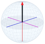 Meaning that, although still a superposition, the qubit is effectively in the first state (ψ₁) because, if measured, the probability of getting that state is 100%. (With 0% probability of getting the ψ₂ state.)
In the Bloch sphere representation, the arrow points straight up with the tip touching the “north pole” of the sphere. As shown in the large image above, we label this point on the sphere |0〉.
This is the equivalent of a binary bit set to zero.
A qubit can also have the exact opposite situation:

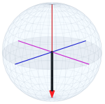 Now a measurement has a 100% chance of getting the ψ₂ state and a corresponding 0% chance of getting the ψ₁ state.
In this case, the arrow in the Bloch sphere representation points straight down with the tip touching the “south pole” — which we label |1〉.
And this is the equivalent of a binary bit set to one.
But remember qubits have the rest of the sphere at their disposal. That, fundamentally, is the quantum qubit difference.
Qubits & Quantum Computing
In quantum computing, we treat the above two states, |0〉 and |1〉, as the quantum computing basis states (somewhat similar to how X and Y axes are the basis for a 2D Cartesian space):

Formally, these two orthogonal basis states are called “ket zero” and “ket one” but casually just “zero” and “one”. [See Bra-Ket Notation for more info on the notation.]
As always, the coefficients (Cₙ) are complex numbers that (when squared) determine the probability of getting that state (|0〉 or |1〉) if the qubit is measured. (When we measure a qubit, we always get one of those two possibilities.)
[Note that, also as always, if a qubit is measured, it “collapses” into the measured state. After a measurement, a qubit is always in the |0〉 or |1〉 state. (Though still in superposition, as described above.)]
There is a relationship between the complex number coefficients, which give us the probabilities of the respective outcomes, and the two angles of the Bloch Sphere:

Evaluating this for the angles theta (θ) and phi (Φ) — given some position of the “state arrow” — gives us the respective C₁ and C₂ (complex) values. (Going the other way is a bit more mathematical and gets us too deep in the weeds for this discussion.)
While the angles theta and phi give us a nice way to visualize the qubit state (especially useful when considering various operations on it), it’s the coefficients that determine the probability of getting a |0〉 or |1〉 result when determining the qubit’s value.
Quantum Computing & Probability
When the qubit is in one of the basis states described above, the outcome is guaranteed, but when both coefficients are nonzero, the outcome is probabilistic based on the (squared) coefficients.
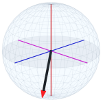 Visually, the state arrow “collapses” to straight up or straight down with a probability based on how close it is to one or the other vertical axis. For example, if the current qubit state was as shown on the right, the odds are high that a measurement gets a |1〉 result and low that it gets a |0〉 result.
But note that a |0〉 result is possible and will occur given enough measurements of a qubit in the same state.
Quantum computation is the process of — for lots of qubits — starting with the arrow in either the reset state |0〉 or in some random state and applying various operations to nudge the arrow closer and closer to the vertical axis reflecting the desired outcome. As in the image just above right.
Entanglement enters the picture here in linking the qubits to nudge them collectively. (For instance, towards providing the prime number factors of a large number and breaking all RSA-encrypted data.)
That quantum computing outcomes are probabilistic means quantum ‘algorithms’ are run thousands of times to determine the most likely outcome(s).
[A quantum ‘algorithm’ is a series of quantum gates that perform various operations on the (entangled) qubits. At a circuit level, regular binary computers also manipulate a series of logical gates, but even the most low-level programming language is far above that level. Quantum computing, for now, remains at the circuit level. Current languages deal with gate operations.]
Physical Qubits
Qubits are two-state systems, so any two-state quantum system is a potential qubit.
One example is quantum spin in particles with spin-½ (such as electrons and silver atoms). Spin is a superposition between two basis states, typically up and down, and these act as the |0〉 and |1〉 states. [See Quantum Spin for details.]
Another example is polarized light — more precisely, polarized photons. Polarization is a superposition between two basis states, for instance horizontal and vertical polarization, and these act as the |0〉 and |1〉 states. [Note that photon polarization is photon spin. See Photon Spin for details.]
There are many other ways to implement qubits physically. For instance, the Josephson junction, a tiny super-conducting micro-circuit. See Qubit: Physical implementation on Wikipedia for a list.
Many Worlds?
I think the combination of ℝ² qubits in superposition plus the entanglement between them does sufficiently explain how quantum computing works.
Our brains distinguish different musical instruments playing the same notes, or different people speaking the same phrase, because these are complex sounds that are superpositions of myriad pure tones. There is an enormous amount of information encoded in such waveforms.
Likewise, quantum states in qubits (which are also described by waves — specifically, wavefunctions). Like sound waves, wavefunctions encode considerable information. Indeed, they encode everything about the system!
A question I have about the MWI of QC is are those other worlds getting the wrong answers? In some cases, seriously wrong. What puts us in the branches with the right answers? [Really just raising the Born rule issue again in the MWI.]
That said, I’m certainly (and firmly) among those who think the MWI doesn’t make any sense and almost certainly isn’t true, so I am not without bias.
§ §
Stay real-squared, my friends! Go forth and spread beauty and light.
∇




November 20th, 2026 at 5:11 pm
Edited this out of the post to keep it slightly less mathematical:
For example, if we’re in the |0〉 state, the arrow points straight up, and the angle theta is zero. The angle phi doesn’t matter because here it just rotates the arrow leaving it pointing the same way.
With theta=0, we have:
Since cos(0)=1 and sin(0)=0, we have:
And we can see why phi doesn’t matter: the right-hand term has a zero, so the whole thing vanishes.
In the other definite state, |1〉, the arrow points straight down, and the angle theta is 180°. Again, the angle phi won’t matter because it would only rotate the arrow.
With theta=180° (aka π radians), we have:
Since cos(π/2)=0 and sin(π/2)=1, we have:
The exponential term, e to the power of i times phi, remains, so |1〉 does have a phase component, but the phase doesn’t change the coefficient.