QM 101: Photon Spin

Earlier in this QM-101 series I posted about quantum spin. That post looked at spin 1/2 particles, such as electrons (and silver atoms). This post looks at spin in photons, which are spin 1 particles. (Bell tests have used both spin types.) In photons, spin manifests as polarization.

Photon spin connects the Bloch sphere to the Poincaré sphere — an optics version designed to represent different polarization states. Both involve a two-state system (a qubit) where system state is a superposition of two basis states.

Incidentally, photon polarization reflects light’s wave-particle duality.

That’s because the polarized light has a classical wave description as well as a quantum description based on photons. Both give the same basic results.

Figure 1. Light waves. The electric field (E, red) and the magnetic field (B, blue) are orthogonal to each other and to the direction of travel.
[image copied from Wikimedia commons]

Considered as an EMF wave, light has an electric field and a magnetic field, which oscillate (wave) in sync, but perpendicular to each other. Both oscillate perpendicular to the direction of travel (which canonically is the Z-axis).

The polarization of the light wave depends on the orientation of the electric field, E, which oscillates in the X-Y plane as it moves in the Z direction. The orientation of the X and Y axes is arbitrary and usually is selected to make the math for a given situation easier. (We ignore the magnetic field, B, because it just “shadows” the electric field.)

If we imagine looking down the Z-axis at on oncoming light beam, we might see something like one of the panels in Figure 2:

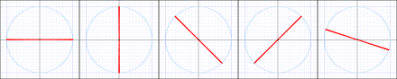
Figure 2. Linear polarization states of a light wave. The first two are typically called horizontal and vertical, respectively. The other three can be viewed as superpositions of the first two.

These panels view the E field edge-on as it waves back and forth. If the angle of the oscillation remains fixed over the cycle, we say the light has linear polarization. We can think of a specific angle of polarization as a polarization state.

Usually context provides a reference establishing a local “up” (and the Y-axis), but the choice is entirely arbitrary. Given some such reference, linear polarization can be horizontal (panel 1), vertical (panel 2), diagonal (panels 3 & 4), or any arbitrary angle (e.g. panel 5).

Note that the angles in the first and second panels are orthogonal to each other. Likewise the third and fourth panels. We can use either pair as basis vectors for a superposition describing all other (linear) polarization angles. In fact we can use any two polarization angles so long as they are orthogonal (different by 90°).

We use the horizontal and vertical polarization basis states |H〉 and |V〉 and then define the two 45° diagonal states, |D〉 and |A〉 (anti-diagonal), as superpositions of opposite phases:

The opposing phases are reflected in the plus and minus signs. The Diagonal adds the two basis components in phase (+) where as the Anti-Diagonal inverts (-) the vertical component.

Figure 3. Horizontal and vertical polarization add to make diagonal polarization.

Figure 3 shows how the in-phase horizontal (red lines) and vertical oscillations (blue lines) combine to create the diagonal |D〉 polarization. In this case both |H〉 and |V〉 basis components go positive and negative in sync.

When the |V〉 component is exactly out of phase (i.e. a 180° difference), then it goes negative when |H〉 goes positive (and vice-versa). This creates the anti-diagonal, |A〉.

By shifting that phase difference, between 0° and 360°, we create any desired angle of polarization (including the original |H〉 and |V〉, which come from phase differences of 90° and 270°).

This means the above definitions of |L〉 and |R〉 are special cases of a single equation:

Where θ (theta) is the phase difference in radians. The coefficients, r, determine the relative mixture of basis states. In the |A〉 state, the 180° phase shift evaluates to multiplying by -1, which is where the minus sign comes from. The |D〉 state, shifted 0°, evaluates to +1. These unity values allow the special case versions.

§

Figure 4. Linear polarization 2D vector space.

We can put together what we’ve got so far (linear polarization of light waves) with Figure 4. It’s a simple 2D version that works somewhat like the Bloch sphere does, although here orthogonal vectors are the more traditional 90° apart.

It’s limited to linear polarization, but one thing that’s nice is that it physically correlates to the actual axes of polarization.

Note that the polarization angle only rotates through 180° (p radians), because a given polarization (say vertical) is the same when rotated 180° (still vertical).

That means the vector representing a given polarization is always in the shaded right half of the circle. Any 180° reflection represents the same polarization (very different from the Bloch sphere where opposing vectors are orthogonal).

The main point here is that we can use |H〉 & |V〉 as basis vectors, or |D〉 & |A〉 or any two orthogonal unit vectors in the right hemisphere. Technically speaking, because -90° is a reflection of +90°, the range is from +90° through less than -90° — mathematically written as [+90°, -90°).

§

Linear polarization is just part of the story. In fact, it’s a special case of elliptical polarization, which is the actual polarization state of light.

If we “fatten” the linear oscillations from Figure 2, we get elliptical oscillations:

Figure 5. Elliptically polarized light. The five panels reflect the five panels in Figure 2. The color spectrum (red-green-blue) shows the phase.

The first four panels above are elliptical versions of the first four panels in Figure 2. Each set illustrates four fundamental modes, horizontal, vertical, diagonal, and anti-diagonal. The fifth panel shows an arbitrary angle.

Notice that the ellipse can be thin or fat. When it thins to a line, we have the special case of linear polarization. It can also fatten into a circle:

Figure 6. Horizontal elliptical polarization expanded to circular. Panels 4 & 5 show Left & Right circular polarization, respectively. Note that circular polarization has no orientation angle.

Which gives us the special case of circular polarization. The color shading (red-orange-green-blue-purple), indicates rotation direction. The last panels show the |L〉 (left circular) and |R〉 (right circular) modes.

In all cases, these elliptical and circular diagrams show the rotation of the electric field during a single cycle. (In linear polarization the field does not rotate during the cycle.) The rotation is due to phase differences. It’s not as if the light source is rotating.

As with the |H〉 & |V〉 states and the |D〉 & |A〉 states, we can use the |L〉 & |R〉 states as basis states for defining all other polarizations. In fact, you’ll see that with regard to photon spin, the |L〉 & |R〉 states are the natural basis states.

§ §

Recall that we’re considering polarization in terms of a view down the Z-axis with the electric field oscillating in the X-Y plane. To describe this we need to account for two degrees of freedom, hence the two basis states.

Mathematically, we can represent polarization states with a Jones vector, which is a two-component (X-Y) vector that uses complex numbers:

Where r is a real number indicating the component’s magnitude, and θ (theta) is the phase in pi radians. Different values of these generate all possible polarization states and angles. Put the opposite way, all polarization states map to some unique Jones vector.

[BTW: thinking about vectors that use complex numbers as components lead to the complex 2D/4D notion I posted about recently. No real connection to Jones vectors, though.]

§

Figure 7. The Poincaré sphere of polarization states. Pure states lie on the surface, the interior contains mixed states.
[Image copied from Wiki]

We can represent all polarization modes graphically using the Poincaré sphere. It’s a specialized version of the Bloch sphere.

As in the Bloch sphere, opposing (antipodal) vectors here are considered orthogonal. Specifically, their inner product is zero.

In the Poincaré sphere, the three pairs of polarization basis states form the three axes. The |L〉 & |R〉 circular states form the vertical axes. The |H〉 & |V〉 linear states form one horizontal axis; the |D〉 & |A〉 linear states form the other.

In general, a horizontal vector represents linear polarization at some angle defined by the vector’s rotation around the vertical axis. A vertical vector, either up or down, represents circular polarization. Any other vector represents some kind of elliptical polarization.

As already mentioned, all points on the sphere are some form of elliptical polarization, but the horizontal and vertical cases are special.

Figure 7 also shows that the three axes are labeled S1, S2, S3, which connect the Poincaré sphere to the Stokes parameters (which also describe light polarization):

Where φ (phi) is the the azimuth, and χ (chi) is the ellipticity.

§ §

Figure 8. Graphic depiction of a right-handed (clockwise) photon spin vector.

The classical wave description is just one half of the duality. In quantum mechanics, light is also a (spin 1) particle — a photon.

Electrons are spin 1/2 particles (fermions) and have a two-state spin on three axes, X, Y & Z.  The spin states are labeled |Up〉 and |Down〉. Measurements on the axes are mutually exclusive. Any given axis can be a basis for defining the other states as superpositions.

In contrast, photons are spin 1 particles (bosons) that spin only on one axis, the direction of travel (the Z-axis). This (circular) quantum spin is either: |Left-handed〉, |Right-handed〉, or a superposition of both.

Photon spin manifests as photon polarization.

As with the wave description (and the Poincaré sphere), any polarization state can be described by a superposition of the |L〉 & |R〉 circular spin basis states:

Any of the basis states described above forms a qubit, which is why both types of spin are of interest in quantum computing. Two-state systems are also the easiest for students (like me!) to study.

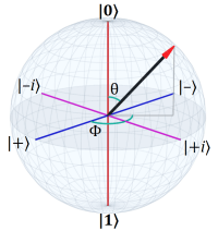
Note that with the following mapping:

• |R〉 = |0〉
• |L〉 = |1〉
• |H〉 = |+〉 — aka 1/√2 ( |0〉 + |1〉 )
• |V〉 = |–〉 — aka 1/√2 ( |0〉 – |1〉 )
• |D〉 = |+i〉 — aka 1/√2 ( |0〉 + i|1〉 )
• |A〉 = |–i〉 — aka 1/√2 ( |0〉 – i|1〉 )

The Poincaré sphere is identical to the Bloch sphere; both describe the same thing. Superpositions of circularly polarized waves of light and superpositions of left- and right-handed photon spins are dual accounts of the same phenomena.

§ §

The two-state qubit nature of photon polarization and that photons can be quantum entangled makes them useful in Bell Tests.

What’s more, polarization is much easier to measure than the up/down property of 1/2 spin particles. Rather than the large magnets of a Stern-Gerlach device, a polarization test just requires a common linear polarization filter. (Scientists use really good ones, of course.)

The Quantum Spin post described how second and third measurements of the same particle demonstrate the nature of wavefunction collapse and non-commuting measurements. Linear photon polarization is the same way.

Think of a linear polarization filter as a venetian blind that passes only light waves that vibrate in the right direction to get through. Ideally the wave should be fully aligned with the slot of the blinds to pass through, but it turns out there is a probability of passing through:

Where I is the light intensity before and after the filter. The angle, θ (theta), is between the incoming light’s (linear) polarization and the filter angle. This is  known as Malus’s law for electromagnetic radiation. It can be viewed as reducing a beam of light by a factor that depends on the linear polarization angle of that light.

For individual photons, the probability is:

Where ρ (rho) is the probability of the photon passing through (rather than being absorbed by) the filter.

When the angle is zero, the cosine is 1.0, and the square of that is also 1.0, so polarized light has a 100% chance of passing through a filter if it’s aligned exactly with. Conversely, the cosine of 90° is 0.0, and the square is also 0.0, so there is zero chance of polarized light passing through.

When the angle is 45°, the cosine is 0.7071+, and the square of that is exactly 0.5, which is a 50% chance of passing. Unpolarized light has an even distribution of different polarizations, the average angle of which is 45° so half of unpolarized light passes through.

§

Let’s consider several simple experiments with filters. The first one involves two filters, both set at a 0° angle:

The photon, γ (gamma), initially has unknown polarization and, thus, a 50% chance of passing through. If it does, it is now linearly polarized at 0° and therefore has a 100% chance of passing through the second filter. On average, 50% of the photons pass through. Those that do are linearly polarized at a 0° angle.

In the second experiment, the second filter is set to 90°:

The first stage here is the same as before. Half the photons pass through the first filter. Those that do are now polarized at 0° and, therefore, none pass through the second filter.

In the third experiment, we add a stage between the first two.

Remember that no photons passed in experiment #2. Here, the second stage has a 45° angle, so the photon has a 50% chance of passing. If it does, its polarization angle is 45°, so it now has a 50% chance of passing the third filter. On average, 12.5% of the photons pass. Those that do are polarized at 90°.

Note that we’ve rotated the original polarization of 0° to 90°. The addition of a third filter not only allows light to pass but rotates the polarization.

That is quantum mechanics in action, and it can be demonstrated with three old polarizing sunglass lens!

§ §

There’s more to say about this, including getting into the mathematics a bit deeper (nothing worse than I’ve covered before). There are some even more interesting experiments with polarizing filters, not to mention how entangled polarized photons are used in Bell tests.

Until next time…

Stay elliptically polarized, my friends! Go forth and spread beauty and light.

∇