 The previous post began an exploration of a key conundrum in quantum physics, the question of measurement and the deeper mystery of the divide between quantum and classical mechanics. This post continues the journey, so if you missed that post, you should go read it now.
Last time, I introduced the notion that “measurement” of a quantum system causes “wavefunction collapse”. In this post I’ll dig more deeply into what that is and why it’s perceived as so disturbing to the theory.
Caveat lector: This post contains a tiny bit of simple geometry.
To begin, mechanics is the study of a system’s dynamics, the forces that act on it, and the resulting motion of that system. There are two important points about classical mechanics: Firstly, it directly corresponds to accessible physical objects. Secondly, it is inherently nonlinear. Both in contrast to quantum mechanics, which involves the mysterious quantum state and is linear.
A bit of history: Classical mechanics begins with Newton’s laws of motion in 1687. One-hundred years later, in 1788, Joseph-Louis Lagrange extended classical mechanics with Lagrangian mechanics. His work introduced the notion of the principle of least action. Almost fifty years after that, in 1833, the great mathematician William Hamilton further extended classical mechanics with Hamiltonian mechanics. He added the notion of a Hamiltonian, a notion also important in quantum mechanics. A key difference between Newton’s formulation and the extensions by Lagrange and Hamilton is that the former is in terms of forces on objects whereas the latter is in terms of a system’s energy.
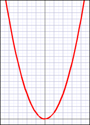
The parabola of x2
For one example of the nonlinearity of classical mechanics we can look at Newton’s famous second law, F=ma, which says that the force (F) on an object is the product of its mass (m) times its acceleration (a).
Mass, at least initially (see below), seems a simple enough property; very roughly speaking, it’s the weight of something.
Acceleration is where the nonlinearity kicks in — it’s the derivative of velocity over time, and velocity is the derivative of distance over time.
Without getting into derivatives, suffice to say that acceleration being the double derivative of distance over time — a quantity we can symbolize as x² — is the nonlinear aspect. Simply put, if we graph x², we get a curve (a parabola).
Linear essentially means a straight line, and a curve isn’t straight, it’s nonlinear.
§
Two asides at this point. Firstly, the theory of gravity, Einstein’s general relativity, is also nonlinear (in part because it has singularities such as black holes). Real-world systems, such as weather and orbits involving more than two bodies, are famously chaotic, and the reason they are is due to the nonlinearity of the equations governing their behavior. We can also consider the parabolic curve of a thrown baseball or fired bullet. The classical world we inhabit, in contrast to the quantum world, seems decidedly nonlinear.
Secondly, while mass seems a simple concept at first blush, Newton’s definition is famously circular. Mass is the density of an object. Density is mass per volume. Oops! Leibniz mocked Newton about this, and it remained a slippery concept until Peter Higgs (and others) came up with the Higgs field (but that’s a story for another time).
§ §
Getting back to the question of measurement, the quantum equivalent of classical laws of motion is the infamous Schrödinger equation (or the relativistic Dirac equation), which say how a quantum state evolves (that is to say, moves).
While we won’t venture into the math, it’s worth a brief look:

There are a several things to notice. Firstly, this is just one form of the equation, there are others. In particular, this is a time-dependent form. The d/dt on the left tells us we’re taking the derivative (of the wavefunction) over time. The Ψ(t) that appears on both sides tells us that we’re looking at the wavefunction Ψ (psi, usually pronounced “sigh”) at some point t in time.
Secondly, a bit more importantly, that little i on the far left is the imaginary unit — the basis of the complex numbers. Its presence is significant in how it seems to require complex math in quantum mechanics. There are classical equations that make use of i, but there it’s a mathematical convenience that can be dispensed with (at the expense of more complicated math). But in quantum math it’s the basis of quantum interference, the existence of which is a crucial difference between quantum and classic mechanics.
(As an aside, quantum interference, quantum superposition, and quantum entanglement, strike me as three key differences between quantum and classical mechanics. We don’t experience them in the classical world.)
Thirdly, as something of an aside, the Ĥ symbol (pronounced “H-hat”) is the Hamiltonian operator that defines the kinetic and potential energy of the system the equation describes. In general, the “hat” symbol over a letter means the letter stands for some form of operator. (See QM 101: What’s an Operator?) A big part of defining a Schrödinger equation for a given system consists of defining its Hamiltonian. (And also, of defining its wavefunction.)
The key to the Schrödinger equation is that it describes the linear evolution of the wavefunction (the quantum state). In practice this means that, given the wavefunction at any time t, we can use the Schrödinger equation to obtain the quantum state at any other time, forward or backward. (Given the typical nonlinearity of classical motion, this is a striking difference about the quantum world.)
§
Which brings us to the measurement problem and why it is such a problem.
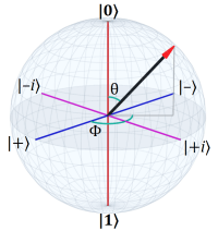
I’ll explore this with a concrete example using a simplified version polarized light. (For a more detailed look, see QM 101: Photon Spin.) Here, I’ll consider only horizontal and vertical polarization, and I’ll forego the more accurate Bloch sphere representation for a two-dimensional representation. (See QM 101: Bloch Sphere.)
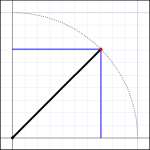
Figure 1: 45°
The polarization angle of a photon can be represented as a combination (technically, a superposition) of horizontal and vertical polarization. Depending on the ratio between them, they can describe any other angle. For instance, equal parts of both result in a 45° polarization. (See Figure 1)
For simplification we can represent this as a quarter-circle where the X-axis is the degree of horizontal polarization, and the Y-axis is the degree of vertical polarization. Here we’ll consider “pure” quantum states, which means the quantum state vector always has a length of one. The points along the quarter-circle are the possible polarization states from fully horizontal to fully vertical.
Note an important aspect of Figure 1: The blue lines project the quantum state onto the horizontal and vertical axes. (The black line is the vector representing the quantum state. Its end point, the red dot, is the actual quantum state.) Basic trigonometry tells us these lines meet the axes at the cosine (horizontal) and sine (vertical) of the angle. Those values are, respectively, cos(45°)=0.707 and sin(45°)=0.707 — the equal parts mentioned above.
Most crucially, the projections of the state (vector) onto the axes represent possible measurements we could make with horizontal or vertical polarizing filters.
§
That last sentence is the heart of this post, and it requires some unpacking before we can get at the measurement problem.
Firstly, in terms of measurement, we’re saying we measure only the horizontal or vertical polarization. This is the basis of our measurement. We can, of course, set a polarization filter at any angle, and that would give us a different basis. All the logic that follows below would still apply.
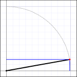
Figure 2: 10°
In picking a basis we want to use orthogonal axes that span the space of possible states. As just mentioned, any polarization angle can be defined as a superposition of the basis axes. For example, an angle of 10° (see Figure 2), would be a superposition of horizontal=cos(10°)=0.985 and vertical=sin(10°)=0.174.
Note that in the case of strictly horizontal polarization (0°) we have cos(0°)=1.0 and sin(0°)=0.0. In the case of strictly vertical polarization (90°) we have cos(90°)=0.0 and sin(90°)=1.0. Thus, even these states are, in fact, superpositions and projections onto the respective axes.
Secondly (still unpacking here), given a photon polarized at 45°, the square of the projection onto an axis gives the probability that we’ll measure the photon. By “measure the photon” I mean that the photon will pass through the filter aligned with that axis and be detected by some device on the other side of the filter.
Why the square of the projection value? Because in less simplified situations the projection can fall onto a negative part of the axis, and there is no such thing as a negative probability. Squaring eliminates negative probability (and, by the way, matches what we see experimentally).
In general, this is the Born rule. The probability of getting some measurement is the square of the projection of the quantum state onto some measurement basis axis.
Looking back at Figure 1, we had projection values of 0.707 for both axes. If we square that, we get 0.50 — a 50% probability the photon will pass a horizontally or vertically aligned filter.
In the case of Figure 2 and 10° polarization, squaring the 0.985 and 0.174 projection values gives us 0.97 and 0.03, which are probabilities of 97% and 3%, respectively. Note that these probabilities must always sum to one.
(In the cases of strictly horizontal or vertical polarization, obviously we end up with 100% and 0% probabilities.)
§ §
We’re finally ready to understand the measurement problem! There are two aspects to it.
Firstly, when we make a measurement, we get a definite result, and the quantum state becomes known. If the photon passes a horizontal filter, then that photon is now horizontally polarized. If it passes a vertical filter, it’s vertically polarized.
This change, in violation of the linear Schrödinger equation, is nonlinear. If we take the Schrödinger equation as fully describing quantum state evolution, then we’re left scratching our heads and wondering what happened. How do we describe this nonlinear change? For that matter, how did nonlinearity even enter linear quantum mechanics?
[For more about how passing through polarization filters changes the polarization state, see QM 101: Fun with Photons.]
Secondly, note that the projection — except in the cases of strictly horizontal or vertical polarization — does not have a length of one. To go on describing the quantum state, we must also make the nonlinear (and rather by fiat) change of setting the vector back to a length of one.
If we put our faith in the Schrödinger equation and the linearity of quantum mechanics, we have an unsolved, and very vexing, problem. One alternative is to view the Schrödinger equation, and even quantum mechanics as currently understood, as an incomplete answer.
§ §
Which would be my view. I think that the lack of unification with gravity, the background dependence, and even the linearity, all suggest we’ve gotten this wrong. (I’m willing here to conflate incomplete with wrong.)
I compare it to the Ptolemaic view of the solar system. Keep in mind that Ptolemy’s geocentric view worked very well for over 1000 years. We might also consider how Newton’s laws worked extremely well for over 200 years until Einstein came up with general relativity.
Quantum mechanics is about 100 years old, and it’s one of the most successful theories we know. Unfortunately, general relativity is the other most successful theory we know, and they’re incompatible on several levels (linear vs nonlinear; background dependent vs GR is the background; quantum vs smooth).
Bottom line, I think faith in quantum mechanics as it now stands may be misplaced.
§ §
For more musings on wavefunction collapse, see the paired Wave-Function Collapse and Wave-Function Story posts from May of 2020 and BB #73: Wavefunction Collapse from August of 2021. They may not add much, but you may find them interesting.
Next time I’ll talk about decoherence and what it has to do (or doesn’t) with the measurement problem.
Stay collapsed, my friends! Go forth and spread beauty and light.
∇


April 4th, 2022 at 7:40 am
We can skip the sine and cosine trigonometry and, instead, use Pythagoras’s famous theorem for the length of the hypotenuse of a right-triangle:
Since we set the state vector to one and use orthogonal axes, the state vector is the hypotenuse of a right-triangle formed by the X and Y axes. This gives us:
Which describes the points of a circle having a radius of one. Note that, now the probabilities, the squares of the projections onto the axes, fall naturally out of the equation. Since the equation applies to all points on the circle — all (pure) quantum states — and applies to any two-state quantum system we describe with a two-dimensional circle.
The notion generalizes to cases with more dimensions, for example a 3D sphere:
Which gives us the projections of any point on the sphere (again, a pure quantum state with three possible measurements), and the squares of those projections are the probabilities of getting each of the three possible measurements. (And, of course, the wavefunction would “collapse” to the measured axis if the measurement succeeded. (If it didn’t, in that case, the quantum state would still be a superposition of some combination of the other two axes.)
The generalization continues to any hypersphere with any number of axes. For instance, with four axes:
And so on.
April 4th, 2022 at 8:04 am
A detail I ignored in the post, but brought out by the comment above, involves what happens if the measurement fails. I ignored it in the post because, if a photon doesn’t pass through the polarizing filter, that means it was absorbed by (an electron in) the filter and, therefore, effectively lost.
If a photon does pass through the filter, we know its wavefunction “collapses” — its polarization angle now matches the angle of the filter. In the cases where it doesn’t, it’s still “collapsed” but collapsed such that its polarization angle matches the orthogonal axis. This behavior is more apparent in other types of experiments where the quantum state isn’t destroyed by being absorbed.
But it’s that “collapse” to the other axis that’s why the probabilities must always sum to one. Upon measurement, there is always a definite result, and in two-state systems, of the measured axis fails, then the “collapse” is necessarily to the other available axis.
That’s why, in systems with more than two states, a measurement that fails results in a “collapse” to some superposition of the other axes.
April 4th, 2022 at 10:54 am
I have a question, nothing to do with this post, regarding light and the human eye’s ability to receive it.
Given rods and cones, where cone cells are charged with converting wavelengths of light to colors, how does white light work?
We can see red, green & blue light, and white light being composed of those three colors (basically), does that mean that “white” light is actually the triggering of three different cones? That is, are cones dedicated to certain colors? Or do cones interpret wavelengths? And if white light is many wavelengths…?
In light of this (ha), what’s your opinion on dark screens vs light ones?
Given what I’ve read about the eye and its light interpretation — dark-mode is NOT the panacea it’s sold to be. I don’t use it. We’re not nocturnal creatures. We expect to see dark things on light backgrounds as part of our evolution.
April 4th, 2022 at 12:22 pm
Color is one of my favorite topics, so pardon me while I blather on a bit!
Let me first differentiate between two different kinds of “white” light. Normal white(-ish) light from incandescent lightbulbs or the sun contains photons of all the (visual) frequencies. Natural white light is the visual equivalent of white noise, sound containing all the (audible) frequencies. “White” light on a computer monitor, however, as you probably know, comes from a blend of red, green, and blue pixels. Some kinds of artificial light, fluorescents, some early LED types, are very spikey in terms of their color curves. (If you’ve ever seen sodium vapor lights, those are essentially monochromatic orange-yellow.)
The reason computer monitor “white” looks white to us is because humans have three types of cones, casually referred to as the “blue”, “green”, and “red”, cones. (Technically, they’re called “S”, “M”, and “L”, respectively for short, medium, and long, wavelengths.) Each type responds to a range of frequencies roughly centered on blue, green-ish, and red-ish. So, it’s not necessary for monitors to attempt to make “white” by combining all the frequencies the way natural sources do. They can use the red, green, and blue, pixels to stimulate the three types of cones.
In fact, the cone responses are a bit on the sloppy side:
The close overlap between the green and red cones, when genetic variation closes the overlap, is responsible for some common types of color-blindness. (Dichromatic lens can help correct it by adding a notch filter between the cones to help separate the responses to green-ish and red-ish light.)
That we have those three types of cones is why TVs, monitors, and color photos, only need to deal with red, green, and blue, in varying proportions to create any color. One of the weirder technological inventions is glass that filters out only the specific frequencies used by these devices. Such glass is sometimes used in glass-walled conference rooms for privacy. Most things look normal through the glass because most things, even if they’re a single color, contain ranges of frequencies, so the strong notching of RGB doesn’t really affect how we see them. But computer monitors and TVs and phone screens, using only those blocked frequencies, look black. Very strange to see in action. People sitting around staring raptly at a black screen.
I’m not a fan of dark screens. I see it as generally a triumph of style over sense. We use white paper and black ink because it works. I started setting my editors to black on white as soon as that capability came around. (I go back to the early days of green on black.) That said, there is some difference between white paper reflecting light and a screen that basically is a light. If your brightness levels are too high, it can cause eye-fatigue, which is why black screen became a thing in the first place. (There is also that some screens are a blue-ish white, and blue light signals your eye that it’s daytime, so staring at a white screen in the evening can interfere with sleep cycles. Modern screens often have an “evening” or “night” mode where they shift to a warmer (red-ish) white to avoid this.
April 4th, 2022 at 7:38 pm
Beautiful. Thanks.
April 7th, 2022 at 7:07 am
[…] the last two posts (Quantum Measurement and Wavefunction Collapse), I’ve been exploring the notorious problem of measurement in quantum mechanics. This post […]
April 7th, 2022 at 10:10 am
Speaking of collapse, I’m a little “collapsed” with regard to this series. I mean that I’m a bit tired of writing about it, so I may take a short break for other things and other posts before I come back to it.
April 10th, 2022 at 7:28 am
[…] the last three posts (Quantum Measurement, Wavefunction Collapse, and Quantum Decoherence), I’ve explored one of the key conundrums of quantum mechanics, the […]
April 13th, 2022 at 4:21 pm
[…] the last four posts (Quantum Measurement, Wavefunction Collapse, Quantum Decoherence, and Measurement Specifics), I’ve explored the conundrum of measurement […]
June 7th, 2022 at 1:02 pm
[…] a five-part series about the measurement problem in quantum mechanics (see Quantum Measurement, Wavefunction Collapse, Quantum Decoherence, Measurement Specifics, and Objective […]
June 23rd, 2023 at 7:09 am
[…] weirdness isn’t in the collapse (well, that too) but in the superposition of physical reality. How can matter coincide? What about […]
February 14th, 2024 at 1:20 pm
[…] As an aside, some might argue that, while decoherence clearly plays a role, we don’t know quite what to call the process — collapse, reduction, decoherence, Many Worlds branching — because we don’t understand it. It’s a central mystery in quantum mechanics. (Of course, the point of the article is that they think they’re on track to solving it.) But decoherence definitely plays a major role — granting that wavefunction reduction actually does happen [see Wavefunction Collapse]. […]
March 14th, 2024 at 12:19 pm
[…] (correctly!) told me it was uploaded for the Wave-Function Collapse post, but I misread it as the Wavefunction Collapse post from 2022, which doesn’t get into the double-slit experiment at all. Very confused was […]