QM 101: What’s an Operator?

In quantum mechanics, one hears much talk about operators. The Wikipedia page for operators (a good page to know for those interested in QM) first has a section about operators in classical mechanics. The larger quantum section begins by saying: “The mathematical formulation of quantum mechanics (QM) is built upon the concept of an operator.”

Operators represent the observables of a quantum system. All measurable properties are represented mathematically by an operator.

But they’re a bit difficult to explain with plain words.

There are words — precise, exact words that work great if one speaks the lingo. (And of course there’s math.) The trick is finding the larger mass of simpler words that can do almost as good a job.

We started with the notion of a vector space — where we see every point in the space as the tip of an arrow that has its tail at the origin. To that we added the notion of (linear) transformations that change (map) all the vectors to new vectors in the space.

Very simply put, an operator is a mathematical function (something that takes one or more values and returns a value) that accomplishes a given transformation on the space.

Typically, a transforming or mapping function is called an operator if the space in question represents the states of some physical system. The transformation operates on the system states.

So an operator is a function (or something we see as a function) that takes a state, changes it, and returns a new state. (Implicitly, it transforms all the vectors in the space.)

§ §

In the previous post in this series, I introduced a number of basic transforms applicable to a 2D Euclidean space. This time I’ll explore those again focusing on implementing them with operators.

The first one was the trivial Null transform that left the vectors unchanged. I used a simple form of notation to express this:

Last time I used z as the input because I was using the complex plane as the vector space, and z is a canonical variable name for a complex number. From now on, although we’ll continue to use complex numbers, we’ll be dealing in vectors, so the notation will reflect that. A canonical variable name for vectors is v (and u if a second vector is needed).

As written above, we have transformation T which takes a vector v. (As with any transform, we expect it to return a new vector.) The transform is defined as simply the input vector v.

We could just leave it at that, but it doesn’t give us a general case for transforms. The definition works for this transform, but not for any other type. However, because the transforms of interest here are linear transforms, we can use the matrices of linear algebra to implement them.

Doing this requires we express our vectors as column vectors — as matrices with one column and as many rows as there are dimensions. The complex plane has two dimensions, so our column vectors have two rows:

In 3D space they would have three. Quantum mechanics often deals with spaces with a vast number, even an infinite number, of dimensions, so conceptually these vectors can have many rows.

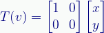
Now we need some square matrix to represent the Null transformation operator. We need a matrix that, when multiplied against the input vector, gives us that same vector. We need the matrix equivalent of multiplying by one, and that’s the identity matrix:

This important matrix exists in as many dimensions as required and consists of all zeros except for ones along the main diagonal. Multiplying this matrix with any other matrix just gives that other matrix.

Now we can write our Null transform like this:

Interested readers are urged to try this. Pick some random values for the x and y members of the vector and do the multiplication.

Now we have a general case for our transforms:

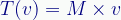
Any operator (transform) can be represented by a matrix M.

§

The Zero transform, which reduced all vectors to the zero vector, I notated as:

We can now define it as:

Again the reader is encouraged to try these, but it should be pretty obvious the result has to be [0, 0].

Note that the original simple definition doesn’t return a vector, but the scalar zero value. I originally defined it as T(z)=[0,0] to make the result a vector but decided to stick to a simpler notation. Our matrix versions always return a column vector.

(There is also that, using that notation, it’s a row vector, and here we’re dealing with column vectors. I didn’t want to muddy those waters.)

§

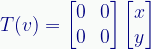
There was also the Real transform, which collapsed the 2D space into a 1D space along the X-axis (the real number line). I notated it as:

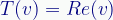
Which, again, returns a real number, not a vector. I could have written it as T(z)=[Re(z), 0], but that seemed too confusing. (It would have been slightly more correct, though.)

We define the matrix version like this:

Readers definitely should try their hand with this one.

I didn’t show you an Imag version that collapses the space to a 1D line on the imaginary axis (the Y-axis). That would have been notated as T(z)=[0, Im(z)], which I thought was even more confusing.

It has a matrix implementation like this:

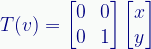
(I did show a similar transform when I scaled the respective axes. See below.)

You may get a sense of what’s going on by comparing these to the identity matrix. Both use one column of that matrix, which preserves one axes, while using zeros in the other column, which (as seen in the Zero transform) collapses the axis.

§

Speaking of scaling, the next transform was scaling the space — which can either enlarge or contract the vectors.

The Scale(0.5) transform.

The notation was:

The simplified notation conceals what is actually a two-step process. As written, the transform takes both a vector, v, and a scaling factor, sf. This implies the transform needs both for each vector it transforms.

That’s redundant and unnecessary. The more accurate way to notate it might be:

Which defines the transform to scale to a certain factor — it’s built in to the definition of the transform, not a required parameter. Note that the free parameter, x, is not defined here but carried through to the transform, which will take a parameter to resolve the missing x with a vector v.

[In more detail: The function Scale, given a scaling factor, returns a new function that scales to that factor. The new function requires (and of course returns) a vector, as all transforms do.]

The matrix version is:

This shrinks the entire space by 0.5. To expand by, say, 1.5:

Note that both reflect the identity matrix, but put the scaling factor where the ones went.

§

Combining the axis collapse and scaling resulted in two transforms I showed last time, ScaleX and ScaleY. These didn’t collapse their axis, just scaled it.

The ScaleY(0.25) transform.

And:

The ScaleX(0.25) transform.

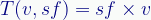
I didn’t show a simple notation for these because there really isn’t one that’s illustrative. The best might be something like (for ScaleY):

Which, even worse than the Real transform, seemed too confusing for the post. Representing these as matrix transforms, however, is easy.

We define ScaleY(0.25) as:

In order to scale the vertical Y-axis by (in this case) 0.25 (as shown in the previous post).

We likewise define ScaleX(0.25) as:

They’re like the overall scaling matrix, but only for one axis. The other column reflects the identity matrix and preserves the axis.

§

The transform matrices (operators!) so far have all been variations on the identity matrix. Because of that, these transforms preserved the orthogonality (right-angles) of the space.

That isn’t true of what I called the Lorentz transform. That operation shifted the space on the diagonal:

The Lorentz(0.5c) transform.

And, again, there isn’t a useful easy notation for it (even more so than with previous examples). But as before, the matrix version is easy:

By easy I mean such a matrix is defined as:

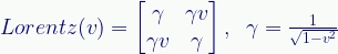
Where v (in this one case in this post) is the velocity relative to c (with 1.0 being c). As I mentioned last time, this transform is the Lorentz transform due to Special Relativity. It’s what we see in a frame moving relative to us.

Doing the math gives us the transform:

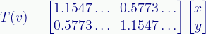
Note that v is once again the input vector here.

§

Another transform I showed was a rotation:

The Rotate(30°) transform.

As with the scaling and Lorentz transforms, we effectively need a function that gives us the matrix we need for a given rotation. (Note that such a “function” can just be knowing how to define the matrix.)

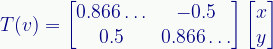
We define a rotation matrix like this:

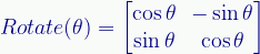
Where theta (θ) is the angle we want to rotate the space. The rotation shown above is 30° so, doing the math, the matrix transform is:

Note that we can scale the rotation by multiplying those matrix numbers by a scaling constant.

I covered matrix-based rotations extensively in two previous posts: Matrix Rotation and Matrix Magic. Refer to those posts for more about rotation using matrices.

§

The final transform is a shear transform:

A Shear transform.

A shear, as with the Lorentz transform, doesn’t preserve right angles. (But, as with all linear transforms, it does preserve straight lines.)

Shear transforms come in too many varieties for a canonical form. The one above looks like this:

You can make sense of this by using what the Matrix Rotation and Matrix Magic posts explained about the i-hat and j-hat column vectors.

I’ll also again point you to Grant Sanderson’s Linear Algebra playlist on his outstanding ThreeBlueOneBrown YouTube channel.

§ §

I’ll revisit the use of matrix operators when this series gets more into quantum computing because “logic gates” in QC are defined as matrices. (They’re also important with regard to quantum spin.)

Next time I’ll get into eigenvectors and eigenvalues.

Stay operating, my friends! Go forth and spread beauty and light.

∇