February 17, 2021

Sideband #71: Matrix Math

There are many tutorials and teachers, online and off, that can teach you how to work with matrices. This post is a quick reference for the basics. Matrix operations are important in quantum mechanics, so I thought a Sideband might have some value.

I’ll mention the technique I use when doing matrix multiplication by hand. It’s a simple way of writing it out that I find helps me keep things straight. It also makes it obvious if two matrices are compatible for multiplying (not all are).

One thing to keep in mind: It’s all just adding and multiplying!

Let’s start with the basics: A matrix is a rectangular bundle of numbers. Being rectangular, it has rows and columns, the number of each being the main characteristic of a matrix. Rows are always listed first, so a 3×1 matrix has three rows and one column, while a 2×2 matrix has two of each.

A matrix with the same number of rows and columns (such as a 2×2 matrix) is a square matrix, which is special.

Two other important special matrix types are column vectors, which have multiple rows, but just one column (their size is n×1); and row vectors, which have multiple columns, but just one row (size 1×n). In either case, the column or row of n numbers is treated as a vector.

The idea of number bundles isn’t new; the vectors just mentioned are bundles of numbers. Even a complex number is a number bundle; it has a real part and an imaginary part. (That it has two parts is what let us treat it as a 2D vector.)

Matrices have many uses in mathematics. They are a type of number, so, as with all numbers, there are operations on matrices that create new matrices or return others types of numeric values. For instance, a matrix can have an inner product, which is an operation that returns a single numeric value.

Specifically, we can add and multiply matrices, but there are some constraints.

Matrix addition requires that both matrices be the same size; that is, they must have the same number of rows and columns. Then, just as with vector addition, matrix addition is just a member-wise add that results in a sum matrix (also of the same size).

$A+B=\begin{bmatrix}a_{11}&a_{12}\\a_{21}&a_{22}\end{bmatrix}+ \begin{bmatrix}b_{11}&b_{12}\\b_{21}&b_{22}\end{bmatrix}= \begin{bmatrix}a_{11}+b_{11}&a_{12}+b_{12}\\a_{21}+b_{21}&a_{22}+b_{22}\end{bmatrix}$

This generalizes to any number of rows and columns.

Matrix addition is both associative…

(A+B)+C = A + (B + C)

…and commutative…

A+B = B+A

Matrix multiplication is (notoriously) a little more complicated.

While, like addition, it is associative, it is not commutative:

A×B ≠ B×A

The order of multiplication matters and is a factor in the constraint. The rule is that the column count of the matrix on the left must match the row count of the matrix on the right.

The by-hand technique highlights this:

The idea is simply to write the second (right-hand) matrix above, thus leaving a space to do the calculation. It lines thing up nicely, and if you want, you can move the second column of the above matrix more to the right to place it over the calculations that use that column (I usually don’t bother).

Notice how this also helps illustrate why the column count of the left-hand matrix must match the row count of the right-hand one.

We can make the order of operation more obvious by converting the square matrix to a row or column vector that itself contains vectors:

Each of the components is a vector with two elements. The arrow over the name indicates a vector. Now we can visualize the multiplication like this:

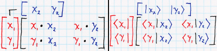
On the left side, the column and row vectors, each containing vectors. On the right side, the same thing in bra-ket notation (which I’ll explore in more detail in another post).

In either case, what we’re doing is taking the inner (or dot) product of the component vectors. The inner product is a multi-dimensional form of multiplication (of taking a scalar product of two numbers), so we’re doing the same multiplication as shown in the first version, but these versions better illustrate which rows and columns to combine.

Following are some examples of multiplying matrices of different sizes.

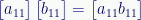
[1×1] times [1×1]

The simplest possible matrix (hardly a matrix at all) is a 1×1 matrix.

The result is a 1×1 matrix, and the single value is the same as we’d get multiplying two scalars together:

$\begin{bmatrix}a_{11}\end{bmatrix}\begin{bmatrix}b_{11}\end{bmatrix} = \begin{bmatrix}a_{11}b_{11}\end{bmatrix}$

But note that a 1×1 matrix is not a scalar. (The difference becomes apparent in the next two cases.)

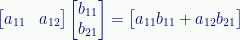
[1×1] times [1×2]

Similar to the first case, the 1×1 matrix acts as a scalar, and the result is the same 1×2 matrix (row vector) we’d get multiplying the 1×2 matrix by a scalar.

$\begin{bmatrix}a_{11}\end{bmatrix}\begin{bmatrix}b_{11}&b_{12}\end{bmatrix}=\begin{bmatrix}a_{11}b_{11}&a_{11}b_{12}\end{bmatrix}$

This effectively is the same as:

$\kappa\begin{bmatrix}b_{11}&b_{12}\end{bmatrix}=\begin{bmatrix}{\kappa}\;b_{11}&{\kappa}\;b_{12}\end{bmatrix}$

But note that, unlike the scalar multiplication, the matrix multiplication cannot be reversed because [1×2][1×1] is an illegal operation. The number of columns in the first matrix doesn’t match the number of rows in the second.

So a 1×1 matrix is not (always) the same as a scalar!

[2×1] times [1×1]

Here’s the legal version of putting the “scalar” matrix second. In this case, the single column of the 2×1 matrix (a column vector) matches the single row of the 1×1 matrix:

$\begin{bmatrix}a_{11}\\a_{21}\end{bmatrix}\begin{bmatrix}b_{11}\end{bmatrix}=\begin{bmatrix}a_{11}b_{11}\\a_{21}b_{11}\end{bmatrix}$

This is the same as:

$\begin{bmatrix}a_{11}\\a_{21}\end{bmatrix}\kappa=\begin{bmatrix}a_{11}\;{\kappa}\\a_{21}\;{\kappa}\end{bmatrix}$

However, as in the second case, this operation cannot be reversed (due to the column/row mismatch), whereas with the scalar operation it can.

[1×2] times [2×1] (inner product)

Multiplying a row vector by a column vector results in a 1×1 matrix usually treated as a scalar:

$\begin{bmatrix}a_{11}&a_{12}\end{bmatrix}\begin{bmatrix}b_{11}\\b_{21}\end{bmatrix}=\begin{bmatrix}a_{11}b_{11}+a_{12}b_{21}\end{bmatrix}$

This operation is known as the inner (or dot) product of the matrices. It generalizes to row and column vectors of larger sizes (so long as they match). When taken as an inner product, the result is always considered a scalar value.

[2×1] times [1×2] (outer product)

Multiplying a column vector by a row vector results in a matrix with as many rows and columns as the vectors (in this case, a 2×2 matrix):

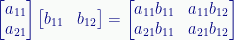
$\begin{bmatrix}a_{11}\\a_{21}\end{bmatrix}\begin{bmatrix}b_{11}&b_{12}\end{bmatrix}=\begin{bmatrix}a_{11}b_{11}&a_{11}b_{12}\\a_{21}b_{11}&a_{21}b_{12}\end{bmatrix}$

This operation is known as the outer product of the matrices. It generalizes to column and row vectors of larger sizes (so long as they match). Note this operation always creates a square matrix.

[2×2] times [2×2]

Multiplying two (same-sized) square matrices results in a new matrix of the same size (in this case, 2×2).

$\begin{bmatrix}a_{11}&a_{12}\\a_{21}&a_{22}\end{bmatrix}\begin{bmatrix}b_{11}&b_{12}\\b_{21}&b_{22}\end{bmatrix}=\begin{bmatrix}a_{11}b_{11}+a_{12}b_{21}&a_{11}b_{12}+a_{12}b_{22}\\a_{21}b_{11}+a_{22}b_{21}&a_{21}b_{12}+a_{22}b_{22}\end{bmatrix}$

(Multiplying square matrices is what many think of as “matrix multiplication” but as the examples above show, it’s not the only form.)

[2×2] times [2×1]

One of the more important examples is multiplying a square matrix times a column vector. In quantum mechanics, square matrices represent operators and column vectors represent quantum states. The output of such an operation is a new column vector, a new quantum state:

$\begin{bmatrix}a_{11}&a_{12}\\a_{21}&a_{22}\end{bmatrix}\begin{bmatrix}b_{1}\\b_{2}\end{bmatrix}=\begin{bmatrix}a_{11}b_{1}+a_{12}b_{2}\\a_{21}b_{1}+a_{22}b_{2}\end{bmatrix}$

Note that you cannot multiply such an operator with a row vector because the column-row counts don’t match.

§ §

Square matrices are special because they have special properties.

An easy one is the trace, which is defined only for square matrices. The trace is the sum of the numbers on the main diagonal.

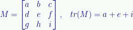
${M}=\begin{bmatrix}a&b&c\\d&e&f\\g&h&i\end{bmatrix},\;\;\;tr(M)=a+e+i$

The main diagonal starts at the upper left and extends down to the lower right. The identity matrix, which is an important matrix, is all zeros except for ones on that diagonal:

$\mathbb{I}=\begin{bmatrix}1&0&0\\0&1&0\\0&0&1\end{bmatrix}$

The identity matrix has the property that using it to multiply another matrix gives that matrix.

${M}\times\mathbb{I}=M$

It’s the matrix equivalent of multiplying a regular number by one, the multiplicative identity.

Multiplying a regular number, n, by its inverse, 1/n, equals one. Similarly, multiplying a matrix by its inverse matrix gives the identity matrix:

${M}\times{M}^{\small{-1}}=\mathbb{I}$

I’ll note that determining a matrix’s inverse is, in many cases, non-trivial. It’s not just a matter of 1/n as with scalar values. (It’s not that hard, just takes a bit of figuring.)

The matrix determinant is, among other things, the scaling factor of the linear transformation the matrix represents.

Given some rectangular area before the transformation, the matrix determinant is how much that area shrinks or grows in the transform. If the determinant is 1, the scale of the space doesn’t change. If the determinant is negative, the transformation somehow inverts (“flips”) the space.

Calculating the determinant for a 2×2 matrix is easy:

${M}=\begin{bmatrix}a&b\\c&d\end{bmatrix},\;\;\;\det(M)=(ad)-(bc)$

The formula for a 3×3 matrix isn’t hard, just long: (aei)+(bfg)+(cdh)-(afh)-(bdi)-(ceg). It looks random and difficult to ever remember, but there’s a rationale and a pattern that, once learned, makes it easy to remember.

A square matrix can have a dot product (two, actually, depending on whether we consider it holding row vectors or column vectors as we did above). The matrix is orthogonal if the dot product is zero (because its vectors are orthogonal).

Taking it one step further, if the vectors are normalized and orthogonal, the matrix is orthonormal.

Of great importance in quantum mechanics, a square matrix is Hermitian if it’s equal to its conjugate transpose.

${M}={M}^{\small\dagger}$

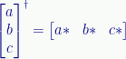
The transpose of a matrix (which can be done to any matrix) is a flip along the main diagonal. Square matrices remain square, of course, but in other matrices the row and column counts switch places. In particular, a transpose converts a column vector to a row vector, and vice versa.

$\begin{bmatrix}a&b\\c&d\end{bmatrix}^{\intercal}=\begin{bmatrix}a&c\\b&d\end{bmatrix}$

The conjugate transpose of a matrix is, first, a transpose, and then taking the complex conjugate of its members. Obviously, this only applies to matrices with complex values.

$\begin{bmatrix}a\\b\\c\end{bmatrix}^{\dagger}=\begin{bmatrix}a*&b*&c*\end{bmatrix}$

[This is important in quantum mechanics, especially with regard to bra-ket notation, where a ket is a column vector, and a bra is a row vector. In particular, bra 〈a| is the conjugate transpose of ket |a〉. The transpose converts the column vector |a〉 to a row vector. Taking the complex conjugate of a is part of the quantum math magic (it’s related to how the magnitude of complex number z is the square root of zz*).]

$\langle{b}\mid{a}\rangle=\begin{bmatrix}b_1*&b_2*\end{bmatrix}\begin{bmatrix}a_1\\a_2\end{bmatrix}$

Lastly (also important in QM), a square matrix is unitary if its conjugate transpose is also its inverse.

${M}^{\small\dagger}={M}^{\small{-1}}\rightarrow{M}\times{M}^{\small\dagger}=\mathbb{I}$

Unitary Hermitian matrices are operators in quantum mechanics (that they are unitary is why QM is said to preserve information).

§ §

This post is just a high altitude fly over to introduce the various aspects of matrix math. Interested parties will obviously have to explore this in more detail.

One point I’ll make about reading (or watching) math topics such as this: It’s not enough to just read or watch. One has to have pen and paper at hand, and one has to do the work. It’s the only way the topic will begin to really make sense. Doing it for yourself is also the only way to really acquire the necessary skill.

Good luck, and I’m always here to help.

Stay in the matrix, my friends! Go forth and spread beauty and light.

∇

⇐ Last Band Next Band ⇒

About Wyrd Smythe

The canonical fool on the hill watching the sunset and the rotation of the planet and thinking what he imagines are large thoughts. View all posts by Wyrd Smythe

This entry was posted on Wednesday, February 17th, 2021 at 7:27 am and tagged with matrix math, matrix multiplication and posted in Math, Sideband. You can follow any responses to this entry through the RSS 2.0 feed.

7 responses to “Sideband #71: Matrix Math”

Wyrd Smythe
February 17th, 2021 at 9:18 am

I wish my penmanship was better. I drew those diagrams more times than I can remember trying to make them look nicer. I don’t know LaTeX well enough to know how to typeset things lined up the right way, and I figured since it’s a by-hand technique anyway…

But I wish my penmanship was better. 😦

Reply
Wyrd Smythe
February 17th, 2021 at 9:24 am

The key take away here is matrix multiplication. The stuff about properties of matrices can come later, but matrix multiplication is a must for working with operators.

This becomes especially important in quantum computing, as QC operations (“quantum gates”) are all represented as matrices.

Interested readers should try for themselves the various multiplication examples I showed using the by-hand technique. Create some matrices with random values and practice multiplying them.

Reply
Wyrd Smythe
February 17th, 2021 at 9:49 am

I saw an article just the other day about non-Hermitian quantum physics. Researchers used quantum computing to simulate it and came up with some interesting results.

One that really caught my eye was:

“The first discovery was that applying operations to the qubits did not conserve quantum information — a behavior so fundamental to standard quantum theory that it results in currently unsolved problems like Stephen Hawking’s Black Hole Information paradox.”

I’ve long been suspicious of the idea that quantum systems conserve information. Unlike conservation of energy or other physical properties, there doesn’t seem to be an associated symmetry underlying the notion of conservation of information. It’s been more an assertion of QM based on the use of unitary operators.

I’ve never fully accepted that it’s a required truth, and these results suggest it might not be.

See: New Physics Rules Tested by Using a Quantum Computer to Create a “Toy-Universe”

Reply
Wyrd Smythe
August 6th, 2021 at 11:16 am

Given some matrix, M, what would we do with:

${e}^{{i}\pi{M}\theta}$

How can a matrix be the exponent of anything, let alone the exponent of e in an expression like that? The trick is to remember that an exponential expression with e is actually a function.

Reply
- Wyrd Smythe
  August 9th, 2021 at 6:43 pm
  
  Reply
- Wyrd Smythe
  August 9th, 2021 at 6:44 pm
  
  😀 😀 😀
  
  Reply
Sideband #72: Trig Is Easy! | Logos con carne
August 6th, 2021 at 11:56 am

[…] want to deal with. (In fairness, it doesn’t pop up much in regular life.) As with matrix math, trig often remains opaque even for those who do have a basic grasp of other parts of […]

Reply