March 15, 2021

QM 101: Bloch Sphere

One small hill I had to climb involved the object I’ve been using as the header image in these posts. It’s called the Bloch sphere, and it depicts a two-level quantum system. It’s heavily used in quantum computing because qubits typically are two-level systems.

So is quantum spin, which I wrote about last time. The sphere idea dates back to 1892 when Henri Poincaré defined the Poincaré sphere to describe light polarization (which is the quantum spin of photons).

All in all, it’s a handy device for visualizing these quantum states.

Any sphere is a three-dimensional object and therefore has an X, Y, and Z, axis. What’s important in this case is that each axis intersects the surface of the sphere at two antipodal points (opposites sides of the sphere). Three axes gives us six points on the sphere.

Even more important is that the surface of the Bloch sphere is the set of all pure quantum states of the system. (The interior of the sphere is the set of all mixed quantum states. For our purposes, only the pure states matter.)

As is typical in geometry, we take the sphere to have a radius of 1 (to simplify the math). There is a unit vector — the quantum state of the system — that moves around inside the sphere, either as the wave-function evolves over time or due to a measurement.

Note that in the former case, the vector moves smoothly and, per the wave-function, completely predictably. It is the latter case that gives quantum physicists the fits — measurement causes the vector to jump to an eigenstate, the dreaded “collapse” of the wave-function.

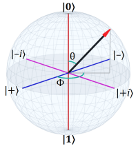
Let’s start with a basic tour of the territory. Below is a larger version of the header image I’ve been using:

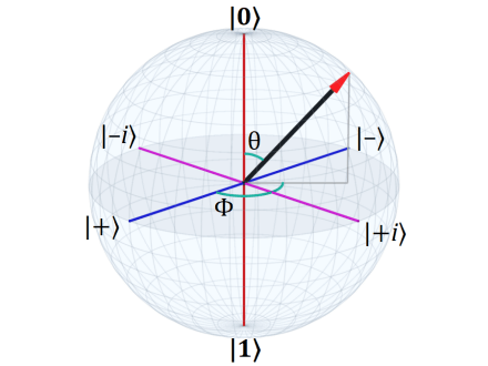
Figure 1. The Bloch sphere, its basis states, and its two angles.

Recall some important points from the Quantum Spin post:

Firstly, a spin or qubit measurement has two outcomes (eigenstates), which we call |0〉 and |1〉 These form the north and south poles (so to speak) of the sphere. This polar axis (red) is canonically defined to be the Z-axis.

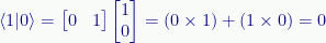
A vital point here is that antipodal vectors, such as |0〉 and |1〉 are orthogonal states! Normally in geometry, orthogonal means two vectors (or even just lines) with a 90° angle, but in the Bloch sphere we define orthogonal to mean two vectors with a 180° angle.

Remember that we define the |0〉 and |1〉 vectors as:

$|{Z}_{+}\rangle=|{0}\rangle=\begin{bmatrix}{1}\\{0}\end{bmatrix},\;\;|{Z}_{-}\rangle=|{1}\rangle=\begin{bmatrix}{0}\\{1}\end{bmatrix}$

For vectors to be orthogonal, their inner product must be zero, and sure enough:

$\langle{1}|{0}\rangle=\begin{bmatrix}{0}&{1}\end{bmatrix}\begin{bmatrix}{1}\\{0}\end{bmatrix}=({0}\times{1})+({1}\times{0})=0$

Secondly, we use these two eigenstates as an eigenbasis that spans all possible states of our system. All other states are superpositions of these basis states.

In particular, we define for the X-axis (blue):

$|{X_+}\rangle=|{+}\rangle=\frac{1}{\sqrt{2}}(|{0}\rangle\!+\!|{1}\rangle)=\frac{1}{\sqrt{2}}\big(\!\!\begin{bmatrix}{1}\\{0}\end{bmatrix}\!\!+\!\!\begin{bmatrix}{0}\\{1}\end{bmatrix}\!\!\big)=\frac{1}{\sqrt{2}}\begin{bmatrix}{1}\\{1}\end{bmatrix}$

And:

$|{X_-}\rangle=|{-}\rangle=\frac{1}{\sqrt{2}}(|{0}\rangle\!-\!|{1}\rangle)=\frac{1}{\sqrt{2}}\big(\!\!\begin{bmatrix}{1}\\{0}\end{bmatrix}\!\!-\!\!\begin{bmatrix}{0}\\{1}\end{bmatrix}\!\!\big)=\frac{1}{\sqrt{2}}\begin{bmatrix}{1}\\{-1}\end{bmatrix}$

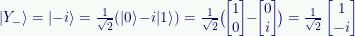
For the Y-axis (purple), we have:

$|{Y_+}\rangle=|{+i}\rangle=\frac{1}{\sqrt{2}}(|{0}\rangle\!+\!{i}|{1}\rangle)=\frac{1}{\sqrt{2}}\big(\!\!\begin{bmatrix}{1}\\{0}\end{bmatrix}\!\!+\!\!\begin{bmatrix}{0}\\{i}\end{bmatrix}\!\!\big)=\frac{1}{\sqrt{2}}\begin{bmatrix}{1}\\{i}\end{bmatrix}$

And:

$|{Y_-}\rangle=|{-i}\rangle=\frac{1}{\sqrt{2}}(|{0}\rangle\!-\!{i}|{1}\rangle)=\frac{1}{\sqrt{2}}\big(\!\!\begin{bmatrix}{1}\\{0}\end{bmatrix}\!\!-\!\!\begin{bmatrix}{0}\\{i}\end{bmatrix}\!\!\big)=\frac{1}{\sqrt{2}}\begin{bmatrix}{1}\\{-i}\end{bmatrix}$

Canonically, the purple Y-axis is aligned with the particle’s motion, The Z-axis and X-axis are perpendicular to it.

Putting that all together:

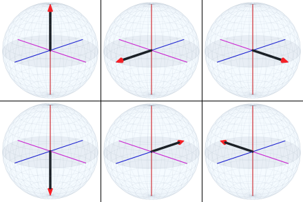
Figure 2. The six eigenstates of the Bloch sphere.

Figure 2 visualizes these six eigenstates by showing the state vector in each of them. On the left, |0〉 and |1〉 (top and bottom); in the middle, |+〉 and |–〉 and on the right, |+i〉 and |–i〉

If we want, we can be more explicit by labeling them (respectively): |Z+〉 |Z-〉 and |X+〉 |X-〉 and |Y+〉 |Y-〉 but the first versions are the more commonly seen.

Note that another common notation, especially when dealing with spin on just the Z-axis is to use |+〉 and |–〉 for |0〉 and |1〉 because |+〉 and |–〉 are more reflective of spin measurements (which have eigenvalues of plus and minus hbar-over-two — the plus and minus being the up and down spin states respectively).

The |0〉 and |1〉 notation is more common in quantum computing because of the similarity to classic bits, 0 and 1. (I also think it’s helpful in differentiating between states and adding or subtracting.)

Here’s another look at the Bloch sphere with the superpositions called out:

Figure 3. The Bloch sphere and eigenstates with their superpositions.

These superpositions should look familiar from the quantum spin post. The Bloch sphere gives us a visualization of those superpositions.

Note that that quantum state vector can touch any point on the sphere’s surface. Remember that the surface of the sphere is the set of all possible pure (normalized) quantum states available to the system.

Where it points at any given time depends on the system and what’s affecting it. For instance, if we make a measurement of spin on the Z-axis, the vector jumps (“collapses”) to either the |0〉 or |1〉 eigenstates (one of the two states shown on the left in Figure 2).

Now let’s talk about those two angles, theta (θ) and phi (Φ).

First consider the general form of a superposition implied by the {|0〉 |1〉} basis:

$|\Psi\rangle=c_1|0\rangle+c_2|1\rangle$

Where the coefficients c are complex numbers. If we write that out explicitly:

$|\Psi\rangle=({a}_{1}\!+\!{ib}_{1})|0\rangle+({a}_{2}\!+\!{ib}_{2})|1\rangle$

Where a and b are real numbers. This implies four degrees of freedom, but quantum mechanics requires they be normalized such that:

$|{c}_{1}|^{2}+|{c}_{2}|^{2}=1$

Because these coefficients are probability amplitudes, and their norm squared must sum to 1. That puts restrictions on their allowed values. For instance, if one is larger, the other has to be smaller. This removes one degree of freedom.

We can then look for a suitable different coordinate system with only three degrees of freedom. A useful choice is the Hopf coordinate system where:

$c_1=e^{i\omega}\cos\frac{\theta}{2},\;\;\;c_2=e^{i(\omega+\phi)}\sin\frac{\theta}{2}$

Plugging the Hopf coordinates into the general superposition gives us:

$|\Psi\rangle=e^{i\omega}\cos\frac{\theta}{2}|0\rangle+e^{i(\omega+\phi)}\sin\frac{\theta}{2}|1\rangle$

Note that:

$e^{i(\omega+\phi)}=e^{i\omega}e^{i\phi}$

So we can extract the global phase, omega (ω), like this:

$|\Psi\rangle=e^{i\omega}\big(\cos\frac{\theta}{2}|0\rangle+e^{i\phi}\sin\frac{\theta}{2}|1\rangle\big)$

Because global phase isn’t physically detectable, we can ignore it, leaving:

$|\Psi\rangle=\cos\frac{\theta}{2}|0\rangle+e^{i\phi}\sin\frac{\theta}{2}|1\rangle$

And now we’re dealing with only two degrees of freedom, the angles theta (θ) and phi (Φ).

As Figure 1 and Figure 3 show, theta is the angle relative to the |0〉 state (the +Z-axis), and phi is the angle relative to the |+〉 state (the +X-axis).

[Note that, in the Hopf coordinate system, theta is restricted to the range 0°–180° while phi has the full circular range 0°–360°. Dividing theta by two effectively reduces its range to 0°–90° which contributes to making |0〉 and |1〉 orthogonal states.]

I sneaked a couple of fastballs over the plate regarding global phase and the Hopf coordinates, so let’s dig into that a little.

Most references to the Hoph coordinate system define the coefficients using three distinct angles:

$c_1=e^{i\phi_1}\cos\theta,\;\;\;c_2=e^{i\phi_2}\sin\theta$

Note there are two angles phi (Φ), one for each coefficient. But above it’s written as:

$c_1=e^{i\omega}\cos\frac{\theta}{2},\;\;\;c_2=e^{i(\omega+\phi)}\sin\frac{\theta}{2}$

This way of writing it is what allows us to factor out one of the exponentials. If we have two distinct values, call them x and y, we can always write them as x and x+n, where n=y–x. (Note that x greater than y means n is a negative number, which is fine.)

To illustrate, if x=45 and y=120, then y–x=75, so x and y can be written as 45 and 45+75. This makes x common to both so we can factor it out (because, in this case, x and y are exponentials).

Therefore the second term can be rewritten:

$|\Psi\rangle=e^{i\omega}\cos\frac{\theta}{2}|0\rangle+e^{i\omega}e^{i\phi}\sin\frac{\theta}{2}|1\rangle$

Which allows us to factor out the first exponential:

$|\Psi\rangle=e^{i\omega}\big(\cos\frac{\theta}{2}|0\rangle+e^{i\phi}\sin\frac{\theta}{2}|1\rangle\big)$

Note that a superposition is a linear sum of the contributing states, which means it is also a state. For any given single state:

$|\psi\rangle=e^{i\phi}|\psi\rangle$

The exponential term is the global phase, and it is not something we can measure or detect. Global phase has no physical meaning, and therefore we can just ignore it.

However, the relative phase between states, and is extremely relevant.

The takeaway here is that, given any two states:

$|\Psi\rangle=e^{i\phi_1}|\psi_1\rangle+e^{i\phi_2}|\psi_2\rangle$

We can always use the n=y–x trick to give us:

$|\Psi\rangle=e^{i\phi_1}|\psi_1\rangle+e^{i\phi_1}e^{i(\phi_2-\phi_1)}|\psi_2\rangle$

And then we can factor out and discard the global phase and consider only the relative phase, Φ₂-Φ₁, between states.

§ §

To finish, let’s consider a few examples of the Bloch angles theta and phi to see what we get. For instance, if θ=0°:

$\cos(0)|0\rangle\!+\!e^{i\phi}\sin(0)|1\rangle=1|0\rangle\!+\!e^{i\phi}0|1\rangle=|0\rangle$

Because cos(0)=1 and sin(0)=0. As you can see, it doesn’t much matter what phi is. Now suppose θ=180° (remember it gets divided by two, so its effective value is 90°):

$\cos(90)|0\rangle\!+\!e^{i\phi}\sin(90)|1\rangle=0|0\rangle\!+\!e^{i\phi}1|1\rangle=e^{i\phi}|1\rangle=|1\rangle$

Because cos(90)=0 and sin(90)=1. Again phi doesn’t matter, but in this case it’s because it has become a global phase.

These two states are both degenerate states in terms of phi. The situation is exactly similar to being at the North or South Pole on Earth. Your longitude has no meaning there.

Now suppose θ=90° and Φ=0° (again keeping mind θ/2):

$\cos(45)|0\rangle\!+\!e^{i{0}}\sin(45)|1\rangle=\frac{1}{\sqrt{2}}|0\rangle+\frac{1}{\sqrt{2}}|1\rangle$

Because e, or any value, to the power of zero is just one. The result should be familiar as the |X+〉 superposition.

I’ll leave the other three as exercises for the dedicated reader.

§ §

In closing, the Bloch sphere is important in quantum computing, because qbits are two-state systems. For example, the IBM Quantum Computer Experience site uses them to visualize how qubits evolve as you work with them.

The Block sphere idea can be extended to systems with more levels, but it becomes an multi-dimensional object we can’t visualize.

What’s probably the most important aspect of this is that classical bits have a single degree of freedom and only two values. A visualization of them would include only the polar |0〉 and |1〉 states with no spherical surface between them. (In fact, classical computers take measures to insure this.)

But qubits can have an infinite range of values between those states, and that is what makes quantum computer so different and, for some applications, so powerful.

Stay spherical, my friends! Go forth and spread beauty and light.

∇

About Wyrd Smythe

The canonical fool on the hill watching the sunset and the rotation of the planet and thinking what he imagines are large thoughts. View all posts by Wyrd Smythe

This entry was posted on Monday, March 15th, 2021 at 7:27 am and tagged with Bloch sphere, QM101, quantum computing, quantum mechanics, quantum spin and posted in Math, Physics. You can follow any responses to this entry through the RSS 2.0 feed.

9 responses to “QM 101: Bloch Sphere”

Wyrd Smythe
March 15th, 2021 at 10:48 am

It’s possible the n=y-x trick is still a little confusing. Here are all the steps…

Given:

$|\Psi\rangle={r}_{1}{e}^{i\theta_1}|0\rangle+{r}_{2}{e}^{i\theta_2}|1\rangle$

Where r₁ and r₂ are real numbers. Then:

$|\Psi\rangle={r}_{1}{e}^{i\theta_1}|0\rangle+{r}_{2}{e}^{i((\theta_2-\theta_1)+\theta_1)}|1\rangle$

Which is the same as:

$|\Psi\rangle={r}_{1}{e}^{i\theta_1}|0\rangle+{r}_{2}{e}^{i(\theta_2-\theta_1)+({i}\theta_1)}|1\rangle$

And therefore:

$|\Psi\rangle={r}_{1}{e}^{i\theta_1}|0\rangle+{r}_{2}{e}^{i(\theta_2-\theta_1)}{e}^{i\theta_1}|1\rangle$

Because:

${e}^{a+b}={e}^{a}\times{e}^{b}$

Which lets us factor out the first exponential:

$|\Psi\rangle={e}^{i\theta_1}\big({r}_{1}|0\rangle+{r}_{2}{e}^{i(\theta_2-\theta_1)}|1\rangle\big)$

And because it’s a global phase, we can discard it:

$|\Psi\rangle={r}_{1}|0\rangle+{r}_{2}{e}^{i(\theta_2-\theta_1)}|1\rangle$

(The real numbers r₁ and r₂ are the normalization constants to insure the probability amplitudes have norms squared that sum to 1.)

Reply
Wyrd Smythe
March 15th, 2021 at 11:08 am

Astute readers might wonder, if θ/2 is a factor in making |0⟩ and |1⟩ orthogonal, why isn’t Φ also divided by 2 to participate in making the the eigenvectors for the other axes orthogonal?

It’s because those eigenvectors are superpositions of the (orthogonal) {|0⟩, |1⟩} basis vectors.

We can do the math to prove that |+⟩ and |–⟩ are orthogonal. Start with the definition of those superpositions:

$|+\rangle=\frac{1}{\sqrt{2}}\big(|0\rangle\!+\!|1\rangle\big)= \frac{1}{\sqrt{2}}\big(\!\begin{bmatrix}1\\0\end{bmatrix}\!+\!\begin{bmatrix}0\\1\end{bmatrix}\!\big)=\frac{1}{\sqrt{2}}\begin{bmatrix}1\\1\end{bmatrix}$

And:

$|-\rangle=\frac{1}{\sqrt{2}}\big(|0\rangle\!-\!|1\rangle\big)= \frac{1}{\sqrt{2}}\big(\!\begin{bmatrix}1\\0\end{bmatrix}\!-\!\begin{bmatrix}0\\1\end{bmatrix}\!\big)=\frac{1}{\sqrt{2}}\begin{bmatrix}1\\-1\end{bmatrix}$

Now calculate the inner product:

$\langle{-}|{+}\rangle=\frac{1}{\sqrt{2}}\begin{pmatrix}\!\begin{bmatrix}1&\!-1\end{bmatrix}\!\begin{bmatrix}1\\1\end{bmatrix}\!\end{pmatrix}=\frac{1}{\sqrt{2}}\big((1\!\times\!{1})+(1\!\times\!{-1})\big)=0$

The inner product of ⟨+|–⟩ is essentially the same, the minus sign just ends up in the column vector rather than the row vector.

Calculating the inner product of |+i⟩ and |–i⟩ is left as an exercise for the reader.

Reply
QM 101: Bra-Ket Notation | Logos con carne
March 23rd, 2021 at 8:04 pm

[…] basically a ket denotes a quantum state. For example, in two-level quantum systems (see: Bloch Sphere and Quantum Spin) we have the canonical […]

Reply
Sideband #73: Complex 4D | Logos con carne
August 6th, 2021 at 6:33 am

[…] I discussed in the Bloch sphere post, a qubit superposition implies four degrees of […]

Reply
Wavefunction Collapse | Logos con carne
April 4th, 2022 at 7:08 am

[…] I’ll explore this with a concrete example using a simplified version polarized light. (For a more detailed look, see QM 101: Photon Spin.) Here, I’ll consider only horizontal and vertical polarization, and I’ll forego the more accurate Bloch sphere representation for a two-dimensional representation. (See QM 101: Bloch Sphere.) […]

Reply
Quantum Decoherence | Logos con carne
April 7th, 2022 at 7:07 am

[…] rotation around the sphere. (The basis vectors are the vertical axes labeled |0〉 and |1〉. See QM 101: Bloch Sphere for […]

Reply
Wyrd Smythe
May 21st, 2022 at 1:38 am

One interesting thing about the Bloch sphere is that it graphically illustrates why quantum computing is so different from, and can be more powerful than, classical computing.

A bit has only two states (and no superpositions). In terms of the Bloch sphere, a bit is two vertical states, |0⟩ and |1⟩, and nothing else. The degrees of freedom finite and limited to those two states.

But a qubit can point to any point on the Bloch sphere, which is R² — not just an infinity, not just an uncountable infinity, but a two-fold uncountable infinity. Qubits have two degrees of (uncountably) infinite freedom.

That’s the power of quantum computing!

Reply
The Power of Qubits | Logos con carne
June 7th, 2022 at 1:01 pm

[…] we have two quantum eigenstates |0〉 and |1〉 that form the basis of a Hilbert space. (See QM 101: Bloch Sphere for details.) The actual state of the system is represented by a unit-length vector that can point […]

Reply
2022: I Hardly Knew Ya | Logos con carne
January 14th, 2023 at 3:09 pm

[…] QM 101: Bloch Sphere (2021, 247) […]

Reply