March 22, 2021

QM 101: Bra-Ket Notation

When I was in high school, bras were of great interest to me — mostly in regards to trying to remove them from my girlfriends. That was my errant youth and it slightly tickles my sense of the absurd that they’ve once again become a topic of interest, although in this case it’s a whole other kind of bra.

These days it’s all about Paul Dirac’s useful Bra-Ket notation, which is used throughout quantum mechanics. I’ve used it a bit in this series, and I thought it was high time to dig into the details.

Understanding them is one of the many important steps to climb.

The notation uses the vertical bar (|) and the angle brackets (〈 and 〉) to construct |kets〉 and 〈bras|.

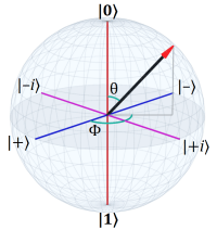
Very basically a ket denotes a quantum state. For example, in two-level quantum systems (see: Bloch Sphere and Quantum Spin) we have the canonical states:

$|0\rangle,\;\;\;|1\rangle$

Which we would refer to verbally as ket zero and ket one, respectively.

Part of the utility of the notation comes from the ability to put anything one wants into a ket. For example, recalling the infamous cat, we might write:

$|Alive\rangle,\;\;\;|Dead\rangle$

Some authors even use the cat icons: |😺〉 and |😿〉 (which I fear risks not being rendered correctly on all systems; they are, respectively, the happy and sad cat icons for those with systems that didn’t know what to do with the Unicode).

The point is that kets can be evocative as well as mathematical. They provide a convenient way to talk casually about quantum states.

When they are mathematical, a ket is a column vector representing a quantum state vector. In a two-level system, the canonical |0〉 and |1〉 states are defined:

$|0\rangle\!=\!\begin{bmatrix}1\\0\end{bmatrix}\!,\;\;\; |1\rangle\!=\!\begin{bmatrix}0\\1\end{bmatrix}$

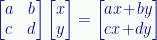
Why vertical column vectors rather than the more familiar horizontal row vectors? Because when we apply an operator to a vector to get another vector, we’re multiplying the vector by a square matrix, and that only works with column vectors:

$\begin{bmatrix}{a}&{b}\\{c}&{d}\end{bmatrix}\begin{bmatrix}{x}\\{y}\end{bmatrix}=\begin{bmatrix}{ax\!+\!by}\\{cx\!+\!dy}\end{bmatrix}$

It’s not a legitimate operation to multiply a square matrix by a row vector:

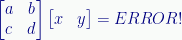
$\begin{bmatrix}{a}&{b}\\{c}&{d}\end{bmatrix}\begin{bmatrix}{x}&{y}\end{bmatrix}=ERROR!$

That’s because matrix multiplication requires the column count of the left matrix match the row count of right matrix. In a two-level system, the operator matrix has two rows and columns, but a row vector has only one row. A column vector has two rows, though, so the multiplication works.

So a ket is a column vector representing a quantum state. The complementary bra is a row vector, but it’s a little more than just that.

Given some ket |a〉, the bra 〈a| is its complex conjugate transpose. Recall that the transpose of a matrix is a flip along its main diagonal, and that the conjugate of a complex number reverses the sign of the “imaginary” part.

For a two-level quantum system:

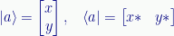
$|{a}\rangle=\begin{bmatrix}{x}\\{y}\end{bmatrix},\;\;\;\langle{a}|=\begin{bmatrix}{x*}&{y*}\end{bmatrix}$

Where x* and y* are the complex conjugates of x and y.

Note that the definitions of both kets and bras are a little more involved mathematically (see the Wiki page), but the above will get one through most of the basic situations. (For instance, it’s enough for everything in this series.)

§ §

So what can we do with kets and bras?

Two of the most common operations are reflected in the canonical representation of a two-level superposition:

$|\Psi\rangle=\alpha|0\rangle+\beta|1\rangle$

Firstly, we can add kets, each a quantum state, to create a new state that is a superposition. This isn’t limited to only two:

For as many as we need. We just add the column vectors. (Which does require that each has the same number of rows, but that is normally the case with multiple states of a given system.)

Secondly, as shown in both examples above, we can multiply a ket by a numeric value (which can be real or complex):

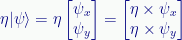
$\eta|\psi\rangle=\eta\begin{bmatrix}{\psi_x}\\{\psi_y}\end{bmatrix}=\begin{bmatrix}{\eta\times\psi_x}\\{\eta\times\psi_y}\end{bmatrix}$

We multiply each component of the column vector by the numeric value. (Using eta (η) as the numeric value is fairly common. It looks a bit like an n, which can stand for normalization constant.)

Another common operation is to take the inner product of two vectors. We do this by converting one of them to a bra:

$\langle{b}|{a}\rangle=\begin{bmatrix}{b_x*}&{b_y*}\end{bmatrix}\begin{bmatrix}{a_x}\\{a_y}\end{bmatrix}=({b_x*}\times{a_x})+({b_y*}\times{a_y})$

Note that the result of this operation is a single numeric value, not a vector. (That value can be complex if the vector components are complex.)

One can think of an inner product as the product (i.e. the multiplication) of two multi-dimensional numbers. When such numbers have just one component (making them essentially ordinary numbers), then the inner product reduces to simple multiplication:

$\langle{a},{b}\rangle=\begin{bmatrix}{a}\end{bmatrix}\begin{bmatrix}{b}\end{bmatrix}=({a}\times{b})$

Note the alternate way of writing the inner product operation: 〈a,b〉. The general form 〈·,·〉 is often used to denote the inner product space.

Another common notation is to use the dot operator: a·b (using the “middle dot” symbol, not the period), because when dealing with vectors, the inner product is sometimes called the dot product.

It’s also sometimes called the scalar product of two vectors — referencing the notion of a product operation and a single numerical result.

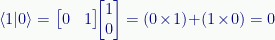
More formally the inner product is, in part, the projection of one vector onto the other. This is especially helpful in determining if two vectors are orthogonal to each other — if they are, their inner product is zero.

For instance, the canonical |0〉 and |1〉 states are orthogonal:

$\langle{1}|{0}\rangle=\begin{bmatrix}{0}&{1}\end{bmatrix}\!\!\begin{bmatrix}{1}\\{0}\end{bmatrix}=({0}\!\times\!{1})\!+\!({1}\!\times\!{0})=0$

The inner product of a vector with itself gives the length (or magnitude) squared of the vector. Given some vector v=(2,3):

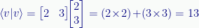
$\langle{v}|{v}\rangle=\begin{bmatrix}{2}&{3}\end{bmatrix}\!\!\begin{bmatrix}{2}\\{3}\end{bmatrix}=({2}\!\times\!{2})\!+\!({3}\!\times\!{3})=13$

Which is the same as the Pythagorean length:

$L^2=x^2+y^2$

So the square root of the inner product of a vector with itself is its length. If the vector is normalized, the length (and its square) are 1.

The term inner product raises an obvious question: Is there an outer product? There is, and it looks like this:

$|{a}\rangle\langle{b}|=\begin{bmatrix}{a_x}\\{a_y}\end{bmatrix}\!\!\begin{bmatrix}{b_x*}&{b_y*}\end{bmatrix}=\begin{bmatrix}{a_x}\!\times\!{b_x*}&{a_x}\!\times\!{b_y*}\\{a_y}\!\times\!{b_x*}&{a_y}\!\times\!{b_y*}\end{bmatrix}$

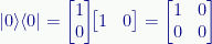
Unlike the inner product, which returns a single numeric value, the outer product returns a square matrix. That means we can use the notation as a convenient way to define operators.

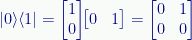
For example, the outer product |0〉〈0| is:

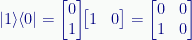
$|{0}\rangle\langle{0}|=\begin{bmatrix}{1}\\{0}\end{bmatrix}\!\!\begin{bmatrix}{1}&{0}\end{bmatrix}=\begin{bmatrix}{1}&{0}\\{0}&{0}\end{bmatrix}$

And the outer product of |1〉〈1| is:

$|{1}\rangle\langle{1}|=\begin{bmatrix}{0}\\{1}\end{bmatrix}\!\!\begin{bmatrix}{0}&{1}\end{bmatrix}=\begin{bmatrix}{0}&{0}\\{0}&{1}\end{bmatrix}$

We don’t have to use the same vectors, we are free to mix and match. For example:

$|{0}\rangle\langle{1}|=\begin{bmatrix}{1}\\{0}\end{bmatrix}\!\!\begin{bmatrix}{0}&{1}\end{bmatrix}=\begin{bmatrix}{0}&{1}\\{0}&{0}\end{bmatrix}$

Or:

$|{1}\rangle\langle{0}|=\begin{bmatrix}{0}\\{1}\end{bmatrix}\!\!\begin{bmatrix}{1}&{0}\end{bmatrix}=\begin{bmatrix}{0}&{0}\\{1}&{0}\end{bmatrix}$

We can also use other values. We’re not restricted to the |0〉 and |1〉 kets.

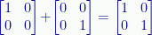
We can combine outer products to create more interesting matrices. For example, if we add |0〉〈0|+|1〉〈1| we get the identity matrix:

$\begin{bmatrix}{1}&{0}\\{0}&{0}\end{bmatrix}\!+\!\begin{bmatrix}{0}&{0}\\{0}&{1}\end{bmatrix}=\begin{bmatrix}{1}&{0}\\{0}&{1}\end{bmatrix}$

We can multiply either or both by a number to create something different. For example:

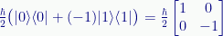
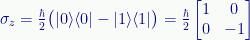
$\frac{\hbar}{2}\big(|{0}\rangle\langle{0}|+(-1)|{1}\rangle\langle{1}|\big)=\frac{\hbar}{2}\begin{bmatrix}{1}&{0}\\{0}&{-1}\end{bmatrix}$

Which is the Z-axis spin operator (see: Quantum Spin).

I wrote it with an explicit -1 to illustrate multiplying one of the outer products by a constant, but a cleaner way (and the usual way) is to subtract the second outer product from the first, which gives us the necessary minus value:

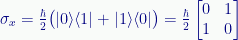
$\sigma_z=\frac{\hbar}{2}\big(|{0}\rangle\langle{0}|-|{1}\rangle\langle{1}|\big)=\frac{\hbar}{2}\begin{bmatrix}{1}&{0}\\{0}&{-1}\end{bmatrix}$

While we’re at it, here is how we can construct the X-axis spin operator:

$\sigma_x=\frac{\hbar}{2}\big(|{0}\rangle\langle{1}|+|{1}\rangle\langle{0}|\big)=\frac{\hbar}{2}\begin{bmatrix}{0}&{1}\\{1}&{0}\end{bmatrix}$

And here how we can construct the Y-axis spin operator:

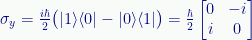
$\sigma_y=\frac{{i}\hbar}{2}\big(|{1}\rangle\langle{0}|-|{0}\rangle\langle{1}|\big)=\frac{\hbar}{2}\begin{bmatrix}{0}&{-i}\\{i}&{0}\end{bmatrix}$

Pay attention to the various combinations and minus signs!

As you can see, a large part of the value of bra-ket notation is due to the ability to so easily represent operations like inner and outer product as well as adding and multiplying by constants.

§ §

One thing we cannot do with two kets is multiply them. For example:

$|{\Psi}\rangle=|{0}\rangle|{1}\rangle$

Is not |a〉 times |b〉, because we cannot multiply two column vectors. For both the column count is one and the row count is two, so there is no way to multiply them. (Lacking a plus sign, nor is it their sum.)

The notation is sometimes used simply to indicate a pair of unrelated quantum states (say two non-entangled particles) in a given system, but it is more often used to describe entangled particles.

In that case, we use the tensor product, which gives us a new column vector with twice as many rows:

$|{ab}\rangle=|{a}\rangle\otimes|{b}\rangle=\begin{bmatrix}{a_x}\!\times\!{b_x}\\{a_x}\!\times\!{b_y}\\{a_y}\!\times\!{b_x}\\{a_y}\!\times\!{b_y}\end{bmatrix}$

I’ll return to this when I post about entanglement.

§ §

As a final note, the angle brackets used in kets and bras are not the less-than and greater-than symbols (‘<‘ and ‘>’).

In HTML, the angle brackets are &lang; and &rang; — the “right angle” and “left angle” symbols .

In the LaTeX system (which is how all the math is implemented in these posts) they are \langle and \rangle.

Their Unicode code points are 10092 and 10093, respectively, or 276C and 276D in hex, so they can also be included in HTML using numerical character references. WordPress insists on converting these, but the generic form starts with &# (for a decimal value) and &#x (for a hex value), then has the numeric value followed by a semi-colon.

For purists, the vertical bar (|), which is an ordinary ASCII code, does also have a Unicode code point close to the angle brackets: 10072 (2758 hex).

Just don’t use the greater-than and less-than symbols. It looks wrong and it is wrong.

Stay bra-ket-ed, my friends! Go forth and spread beauty and light.

∇

About Wyrd Smythe

The canonical fool on the hill watching the sunset and the rotation of the planet and thinking what he imagines are large thoughts. View all posts by Wyrd Smythe

This entry was posted on Monday, March 22nd, 2021 at 7:27 am and tagged with bra-ket notation, inner product, matrix multiplication, outer product, QM101, quantum mechanics and posted in Math, Physics. You can follow any responses to this entry through the RSS 2.0 feed.

7 responses to “QM 101: Bra-Ket Notation”

Wyrd Smythe
March 22nd, 2021 at 8:58 am

That’s pretty much the last of the QM-101 topics I had planned There is the subject of entanglement, but that might end up being part of posts about Bell’s experiments (which use and demonstrate entanglement). Those experiments are the ultimate goal of this series (and might be a couple or three weeks off).

If there are any other topics (or any questions), now would be the time to suggest them (or ask them).

Reply
SelfAwarePatterns
March 22nd, 2021 at 4:35 pm

Excellent job, on this and the entire series! This explanation matches what I’ve read before about Bra-ket notation.

My question though is what it means in terms of the physics to use a bra instead of a ket? Or if we’re converting a ket into a bra just to take the inner or outer product, what does that mean in terms of the physics? (I’ve read enough about entanglement to glean why tensor products are useful.)

No worries if this is a bottomless rabbit hole you’d rather not go down.

Reply
- Wyrd Smythe
  March 22nd, 2021 at 6:00 pm
  
  Thank you! It’s been a good exercise for me, trying to find a way to explain it sensibly. Goes a long way to helping clarify it in my own mind.
  
  “My question though is what it means in terms of the physics to use a bra instead of a ket?”
  
  It’s just a convenient mathematical notation for representing the inner product operation. The deeper question is your second one:
  
  “Or if we’re converting a ket into a bra just to take the inner or outer product, what does that mean in terms of the physics?”
  
  Geometrically, the inner product is the projection of one vector onto another. One can think of it as sort of casting a shadow. If the vectors are orthogonal, the inner product is zero — the shadow is “straight down” as if the sun was overhead and has no length. The more the two vectors point in the same direction, the longer the shadow one will cast on the other. If they point in exactly the same direction, the shadow has maximum length.
  
  So, inner product is a measure of how close to vectors are to being the same.
  
  In quantum mechanics, the vectors in question would be the current quantum state vector and the eigenvector of some putative measurement that could be made on the system. The inner product is the probability amplitude, and its norm squared is the probability of getting that measurement.
  
  Simply put, the closer the state vector is to a given eigenvector, the greater the probability of getting that eigenvector as a measurement result.
  
  Going a bit further down the rabbit hole, in Euclidean space, “orthogonal” means vectors are at 90°, and it’s easy to visualize that the projection is zero. If the angle is less than 90°, its also easy to visualize how one casts a “shadow” on the other. What’s a bit harder is when the angle is greater than 90° — mathematically (in Euclidean space) one gets the same result, but with a minus sign.
  
  So, imagining normalized vectors with a length of one, starting with vector B being identical to vector A (having an angle of 0°), the inner product is 1.0. As the angle grows towards 90° the inner product decreases towards zero and then grows negative until 180° where it’s -1.0.
  
  Therefore, in Euclidean space, the inner product is also helpful in seeing when two vectors are obtuse, orthogonal, acute, or identical.
  
  However, recalling the Bloch sphere, antipodal vectors (i.e. with an angle of 180°) are defined as orthogonal, so in some sense angles between them can never be obtuse. Therefore the inner product only grows from 1.0 (with identical normalized vectors) to 0.0 (with orthogonal vectors).
  
  As an example, consider the |0⟩ and |+⟩ states:
  
  $\langle{+}|{0}\rangle=\begin{bmatrix}\frac{1}{\sqrt{2}}&\frac{1}{\sqrt{2}}\end{bmatrix}\!\!\begin{bmatrix}{1}\\{0}\end{bmatrix}=(\frac{1}{\sqrt{2}}\times{1})\!+\!(\frac{1}{\sqrt{2}}\times{0})=\frac{1}{\sqrt{2}}$
  
  Which is the probability amplitude of those states. The norm squared is:
  
  $|\frac{1}{\sqrt{2}}|^2=\frac{1}{2}$
  
  And, indeed, we’d expect the probability of getting the |0⟩ state — assuming the system is in the |+⟩ state — to be 1/2.
  
  This is also why we always get the same result making a second identical measurement. Making the first measurement puts the system in a known state, say it is |0⟩, and then the probability amplitude of measuring the |0⟩ state is:
  
  $\langle{0}|{0}\rangle=\begin{bmatrix}{1}&{0}\end{bmatrix}\!\!\begin{bmatrix}{1}\\{0}\end{bmatrix}=({1}\times{1})\!+\!({0}\times{0})=1$
  
  The norm squared, of course, is 1. We’re guaranteed to get the same measurement. On the other hand, the probability of getting the |1⟩ state is:
  
  $\langle{1}|{0}\rangle=\begin{bmatrix}{0}&{1}\end{bmatrix}\!\!\begin{bmatrix}{1}\\{0}\end{bmatrix}=({0}\times{1})\!+\!({1}\times{0})=0$
  
  So it never happens. Measurements between those states will have some non-zero amplitude less than 1.0, and will have some norm squared probability of occurring.
  
  Make sense?
  
  Reply
  - SelfAwarePatterns
    March 22nd, 2021 at 6:17 pm
    
    Thanks! It does. This part is exactly what I needed to see.
    
    So, inner product is a measure of how close to vectors are to being the same.
    
    In quantum mechanics, the vectors in question would be the current quantum state vector and the eigenvector of some putative measurement that could be made on the system. The inner product is the probability amplitude, and its norm squared is the probability of getting that measurement.
    
    Simply put, the closer the state vector is to a given eigenvector, the greater the probability of getting that eigenvector as a measurement result.
Wyrd Smythe
March 24th, 2021 at 10:00 am

As I wrote in the Matrix Math post, one way to break down matrix multiplication is to divide the matrices into row and column vectors:

$\begin{bmatrix}\begin{pmatrix}{a_{11}}&{a_{12}}\end{pmatrix}\\\begin{pmatrix}{a_{21}}&{a_{22}}\end{pmatrix}\end{bmatrix}\times\begin{bmatrix}\begin{pmatrix}{b_{11}}\\{b_{21}}\end{pmatrix}&\begin{pmatrix}{b_{12}}\\{b_{22}}\end{pmatrix}\end{bmatrix}$

And then express them as bras and kets:

$\begin{bmatrix}\langle{a_1}|\\\langle{a_2}|\end{bmatrix}\!\times\!\begin{bmatrix}|{b_1}\rangle&|{b_2}\rangle\end{bmatrix}=\begin{bmatrix}\langle{a_1}|{b_1}\rangle&\langle{a_1}|{b_2}\rangle\\\langle{a_2}|{b_1}\rangle&\langle{a_2}|{b_2}\rangle\end{bmatrix}$

Which may, or may not, be helpful in keeping straight which rows and columns to multiply together.

Keeping in mind that, for instance:

$\langle{a_1}|{b_1}\rangle$

Is:

$\begin{pmatrix}{a_{11}}&{a_{12}}\end{pmatrix}\!\!\times\!\!\begin{pmatrix}{b_{11}}\\{b_{21}}\end{pmatrix}=({a_{11}}\!\times\!{b_{11}})\!+\!({a_{12}}\!\times\!{b_{21}})$

Reply
The Power of Qubits | Logos con carne
June 7th, 2022 at 1:01 pm

[…] known for being where he defines and describes his 〈bra|ket〉 notation (which I posted about in QM 101: Bra-Ket Notation). More significantly, Dirac shows how to build a mathematical quantum theory from the ground […]

Reply
2022: I Hardly Knew Ya | Logos con carne
January 14th, 2023 at 3:09 pm

[…] QM 101: Bra-Ket Notation (2021, 151) […]

Reply