 I originally created this page partly to gain some experience embedding LaTeX in WordPress posts and pages, partly to gain experience rendering math equations using LaTeX, and partly to document my exploration of rotation matrices [see the Matrix Rotation and Matrix Magic posts].
To my surprise, this turned into one of my more viewed pages. Apparently, a number of other people find the topic useful.
[2023/17/01] Given the attention this page has gotten and that I’ve been meaning to update it anyway, I finally got myself a Round Tuit. Added some stuff and moved the quantum gate stuff to the Quantum Qubit Math page.
[2025/06/09] Expanded the text and corrected the subscripts of the 4D matrices to reflect the axes being rotated (as with the 2D and 3D matrices — I never got around to updating the 4D examples).
Note that the following assumes the reader understands the basic idea that, in linear algebra, a transformation matrix changes given vectors into different vectors. As such, they transform (or map) all the points of a vector space to new points (or sometimes the same points).
Note also that this page only addresses rotation matrices — transformation matrices that rotate the vector space around one or more axes.
2D
Let’s start with the most basic rotation: 2D rotation. Think of it as rotating a piece of paper on a tabletop but without lifting the paper off the surface. We give the tabletop has X and Y coordinates. The simplest change is no change, and we represent that most basic transformation with the 2D identity matrix:
![\displaystyle{I}^{2}=\begin{bmatrix}{1}&{0}\\[0.4em]{0}&{1}\end{bmatrix}](https://s0.wp.com/latex.php?latex=%5Cdisplaystyle%7BI%7D%5E%7B2%7D%3D%5Cbegin%7Bbmatrix%7D%7B1%7D%26%7B0%7D%5C%5C%5B0.4em%5D%7B0%7D%26%7B1%7D%5Cend%7Bbmatrix%7D+&bg=f9fbf9&fg=00007f&s=2&c=20201002)
We call it I² because it’s the identity matrix for two dimensional transformations. Specifically, it’s the no-change transformation in two dimensions. It changes all vectors into themselves. As a rotation matrix, it represents a zero-degree rotation — a rotation that doesn’t change anything.
The trick to understanding transformation matrices is to look at their vertical columns as column vectors, one for each basis axis of the space.
In the two-dimensional case we have two vertical column vectors, usually called i-hat and j-hat. These start off as unit vectors along the X-axis and Y-axis. They start off identical respectively to x-hat (1,0) and y-hat (0,1), the unit vectors that define the X and Y axes. (The “hat” symbol denotes a unit vector.)
![\displaystyle{M}^{2}=\begin{bmatrix}\,\hat{i}_{x}&\hat{j}_{x}\\[0.6em]\,\hat{i}_{y}&\hat{j}_{y}\end{bmatrix}](https://s0.wp.com/latex.php?latex=%5Cdisplaystyle%7BM%7D%5E%7B2%7D%3D%5Cbegin%7Bbmatrix%7D%5C%2C%5Chat%7Bi%7D_%7Bx%7D%26%5Chat%7Bj%7D_%7Bx%7D%5C%5C%5B0.6em%5D%5C%2C%5Chat%7Bi%7D_%7By%7D%26%5Chat%7Bj%7D_%7By%7D%5Cend%7Bbmatrix%7D+&bg=f9fbf9&fg=00007f&s=2&c=20201002)
The four matrix values, seen as two column vectors, specify where i-hat and j-hat end up. That’s the key to understanding the transformation. The matrix values determine how those column vectors get transformed. The matrix values are the new values for i-hat and j-hat. (That’s why we don’t use x-hat and y-hat, which might have seemed like obvious choices. Those vectors define the axes and can’t change.)
So, a matrix describes a transformation of a space, in this case the 2D plane. Such a transformation might be a scaling, a rotation, a shear, or some combination. Notably, in all cases, the origin stays the same.
In the case of the identity matrix, i-hat is (1,0) and j-hat is (0,1), which is exactly where they started (identical to x-hat and y-hat). That’s what makes the identity matrix the identity matrix. Nothing changes.
A 2D rotation matrix, for a rotation by some angle theta (θ), looks like this:
![\displaystyle{R}_{xy}^{2}(\theta)=\begin{bmatrix}{\cos\theta}&{-\sin\theta}\\[0.4em]{\sin\theta}&{\cos\theta}\end{bmatrix}](https://s0.wp.com/latex.php?latex=%5Cdisplaystyle%7BR%7D_%7Bxy%7D%5E%7B2%7D%28%5Ctheta%29%3D%5Cbegin%7Bbmatrix%7D%7B%5Ccos%5Ctheta%7D%26%7B-%5Csin%5Ctheta%7D%5C%5C%5B0.4em%5D%7B%5Csin%5Ctheta%7D%26%7B%5Ccos%5Ctheta%7D%5Cend%7Bbmatrix%7D+&bg=f9fbf9&fg=00007f&s=2&c=20201002)
The name, 
The result is a matrix with four values based on the sine and cosine of θ. We can use the following table to give us values for four well-known cases of angle θ:
| 0° | 90° | 180° | 270° | |
| sin θ | 0 | +1 | 0 | -1 |
| cos θ | +1 | 0 | -1 | 0 |
Plugging in the values from the first column, the first 2D rotation matrix, a rotation of zero degrees, looks like this:
![\displaystyle{R}_{xy}^{2}(0)=\begin{bmatrix}{1}&{0}\\[0.5em]{0}&{1}\end{bmatrix}](https://s0.wp.com/latex.php?latex=%5Cdisplaystyle%7BR%7D_%7Bxy%7D%5E%7B2%7D%280%29%3D%5Cbegin%7Bbmatrix%7D%7B1%7D%26%7B0%7D%5C%5C%5B0.5em%5D%7B0%7D%26%7B1%7D%5Cend%7Bbmatrix%7D+&bg=f9fbf9&fg=00007f&s=2&c=20201002)
Which is the identity matrix. A rotation of zero degrees does nothing.
The other three matrices for the table values look like this:
 |
 |
 |
Of course, other angles result in different (non-integer) values. We just need the cosine and sine values of the desired angle.
For instance, a 10-degree rotation matrix looks like this:
![\displaystyle{R}_{xy}^{2}(10)=\begin{bmatrix}{+0.9848}&{-0.1736}\\[0.6em]{+0.1736}&{+0.9848}\end{bmatrix}](https://s0.wp.com/latex.php?latex=%5Cdisplaystyle%7BR%7D_%7Bxy%7D%5E%7B2%7D%2810%29%3D%5Cbegin%7Bbmatrix%7D%7B%2B0.9848%7D%26%7B-0.1736%7D%5C%5C%5B0.6em%5D%7B%2B0.1736%7D%26%7B%2B0.9848%7D%5Cend%7Bbmatrix%7D+&bg=f9fbf9&fg=00007f&s=1&c=20201002)
The values are just cos(10°) and sin(10°) — respectively 0.9848… and 0.1736… — plugged into their appropriate spots in the
(If the sine value itself was negative, then the lower-left value would be negative, and the negative sign in the upper-right would make the value positive. The two sine values in the matrix always have opposing signs.)
Note that the 2D case rotates around the origin. The “axis” of rotation can be thought of as being the Z axis (which doesn’t exist in 2D). This positions the 2D examples as being embedded in 3D space (which, from our 3D perspective, they are). The above limits itself to a strict 2D X-Y and a single mode of rotation, but as we’ll see below, being embedded in higher spaces allows “improper” rotations — reflections!
(A “proper” rotation takes place entirely within the object’s dimensions. Two-dimensional objects are limited to rotations involving X and Y, and three-dimensional objects are limited to rotations involving X, Y and Z. Proper rotations do not change the object itself.)
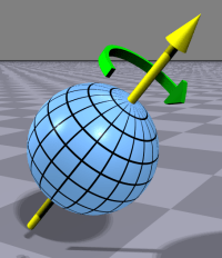
3D
Here’s the 3D identity matrix:
![\displaystyle{I}^{3}=\begin{bmatrix}{1}&{0}&{0}\\[0.5em]{0}&{1}&{0}\\[0.4em]{0}&{0}&{1}\end{bmatrix}](https://s0.wp.com/latex.php?latex=%5Cdisplaystyle%7BI%7D%5E%7B3%7D%3D%5Cbegin%7Bbmatrix%7D%7B1%7D%26%7B0%7D%26%7B0%7D%5C%5C%5B0.5em%5D%7B0%7D%26%7B1%7D%26%7B0%7D%5C%5C%5B0.4em%5D%7B0%7D%26%7B0%7D%26%7B1%7D%5Cend%7Bbmatrix%7D+&bg=f9fbf9&fg=00007f&s=2&c=20201002)
As with the I² matrix, we call this I³ because it’s the identity matrix for three dimensions. As was the 2D version, the 3D identity matrix is the null transformation in 3D. Applying it to a 3D vector just transforms the vector into itself.
In 3D we add a third column vector, k-hat, which conceptually starts off as identical to z-hat, the unit vector defining the Z-axis. We also need a third component, z, for all three column vectors:
![\displaystyle{M}^{3}=\begin{bmatrix}\,\hat{i}_{x}&\hat{j}_{x}&\hat{k}_{x}\\[0.6em]\,\hat{i}_{y}&\hat{j}_{y}&\hat{k}_{y}\\[0.6em]\,\hat{i}_{z}&\hat{j}_{z}&\hat{k}_{z}\end{bmatrix}](https://s0.wp.com/latex.php?latex=%5Cdisplaystyle%7BM%7D%5E%7B3%7D%3D%5Cbegin%7Bbmatrix%7D%5C%2C%5Chat%7Bi%7D_%7Bx%7D%26%5Chat%7Bj%7D_%7Bx%7D%26%5Chat%7Bk%7D_%7Bx%7D%5C%5C%5B0.6em%5D%5C%2C%5Chat%7Bi%7D_%7By%7D%26%5Chat%7Bj%7D_%7By%7D%26%5Chat%7Bk%7D_%7By%7D%5C%5C%5B0.6em%5D%5C%2C%5Chat%7Bi%7D_%7Bz%7D%26%5Chat%7Bj%7D_%7Bz%7D%26%5Chat%7Bk%7D_%7Bz%7D%5Cend%7Bbmatrix%7D+&bg=f9fbf9&fg=00007f&s=2&c=20201002)
As before, the trick is that the imagined transformation vectors (i-hat, j-hat, k-hat) start identical to the basis unit vectors (x-hat, y-hat, z-hat) and are transformed to the values given in the matrix.
Here’s the matrix for 3D rotation involving the X and Y coordinates:
![\displaystyle{R}_{xy}^{3}(\theta)=\begin{bmatrix}{\cos\theta}&{-\sin\theta}&{0}\\[0.6em]{\sin\theta}&{\cos\theta}&{0}\\[0.6em]{0}&{0}&{1}\end{bmatrix}](https://s0.wp.com/latex.php?latex=%5Cdisplaystyle%7BR%7D_%7Bxy%7D%5E%7B3%7D%28%5Ctheta%29%3D%5Cbegin%7Bbmatrix%7D%7B%5Ccos%5Ctheta%7D%26%7B-%5Csin%5Ctheta%7D%26%7B0%7D%5C%5C%5B0.6em%5D%7B%5Csin%5Ctheta%7D%26%7B%5Ccos%5Ctheta%7D%26%7B0%7D%5C%5C%5B0.6em%5D%7B0%7D%26%7B0%7D%26%7B1%7D%5Cend%7Bbmatrix%7D+&bg=f9fbf9&fg=00007f&s=2&c=20201002)
It’s obviously similar to the 
The three matrices for XY rotations of 90°, 180°, and 270° look very much like the three 2D ones above:
 |
 |
 |
The difference being the identity value in the lower-right corner. This represents that the coordinates on the Z-axis do not change. Note also the zeros in the right-most column and lower row. Nothing from the X or Y axes is mixed in with Z during rotation.
Next, here’s the matrix for 3D rotation involving the X and Z coordinates (in other words, around the Y-axis):
![\displaystyle{R}_{xz}^{3}(\theta) = \begin{bmatrix}\cos\theta&{0}&-\sin\theta\\[0.6em]{0}&{1}&{0}\\[0.6em]\sin\theta&{0}&\cos\theta\end{bmatrix}](https://s0.wp.com/latex.php?latex=%5Cdisplaystyle%7BR%7D_%7Bxz%7D%5E%7B3%7D%28%5Ctheta%29+%3D+%5Cbegin%7Bbmatrix%7D%5Ccos%5Ctheta%26%7B0%7D%26-%5Csin%5Ctheta%5C%5C%5B0.6em%5D%7B0%7D%26%7B1%7D%26%7B0%7D%5C%5C%5B0.6em%5D%5Csin%5Ctheta%26%7B0%7D%26%5Ccos%5Ctheta%5Cend%7Bbmatrix%7D+&bg=f9fbf9&fg=00007f&s=2&c=20201002)
The three matrices for XZ rotations of 90°, 180°, and 270° are:
 |
 |
 |
Similar to the XY rotation matrices above, but with the four “rotator” values distributed to the four corner cells. This means the x-hat and z-hat vectors change, but the y-hat vector does not.
Note that, if the 
But if we truncate the 
![\displaystyle{R}_{x}^{2}(\theta)=\begin{bmatrix}{\cos\theta}&{0}\\[0.4em]{0}&{1}\end{bmatrix}](https://s0.wp.com/latex.php?latex=%5Cdisplaystyle%7BR%7D_%7Bx%7D%5E%7B2%7D%28%5Ctheta%29%3D%5Cbegin%7Bbmatrix%7D%7B%5Ccos%5Ctheta%7D%26%7B0%7D%5C%5C%5B0.4em%5D%7B0%7D%26%7B1%7D%5Cend%7Bbmatrix%7D+&bg=f9fbf9&fg=00007f&s=1&c=20201002)
If we apply this to the piece of paper on the tabletop, we get an improper rotation. The y-hat vector is (0,1), so all Y coordinates are mapped to themselves — then don’t change. But the x-hat vector is (cos θ, 0), and cos θ cycles [+1, 0, -1, 0, +1] as θ goes from zero to 360 degrees. When cos θ is zero, all X coordinates map to zero, and the paper becomes a one-dimensional line along its Y coordinates. And when cos θ is -1, the X coordinates are reversed.
So, this improper rotation “collapses” the X coordinates — the width of the paper — to a zero-thickness line along its Y coordinates, then expands it horizontally reversed, then collapses it to vanishing again, and finally expands it back to where it started. In particular, note that an improper rotation of 180 degrees — the halfway point — gives us a reversed, reflected, or backwards version of the object being rotated. In this case, with rotation around the Y axis, we’re lifting the paper from the tabletop in order to rotate it on its Y axis (the lifting is what makes it improper — we’re leveraging a higher dimension). By rotating it 180 degrees, we’re turning it around.
Lastly, here’s the matrix for 3D rotation involving the Y and Z coordinates (rotating around the X-axis):
![\displaystyle{R}_{yz}^{3}(\theta)=\begin{bmatrix}{1}&{0}&{0}\\[0.6em]{0}&{\cos\theta}&{-\sin\theta}\\[0.6em]{0}&{\sin\theta}&{\cos\theta}\end{bmatrix}](https://s0.wp.com/latex.php?latex=%5Cdisplaystyle%7BR%7D_%7Byz%7D%5E%7B3%7D%28%5Ctheta%29%3D%5Cbegin%7Bbmatrix%7D%7B1%7D%26%7B0%7D%26%7B0%7D%5C%5C%5B0.6em%5D%7B0%7D%26%7B%5Ccos%5Ctheta%7D%26%7B-%5Csin%5Ctheta%7D%5C%5C%5B0.6em%5D%7B0%7D%26%7B%5Csin%5Ctheta%7D%26%7B%5Ccos%5Ctheta%7D%5Cend%7Bbmatrix%7D+&bg=f9fbf9&fg=00007f&s=2&c=20201002)
The three matrices for YZ rotations of 90°, 180°, and 270° are:
 |
 |
 |
Again, similar to the ones shown above, but now the “rotators” are in the lower right four matrix positions, and it’s the x-hat vector that doesn’t change.
If we again consider a version truncated for 2D:
![\displaystyle{R}_{y}^{2}(\theta)=\begin{bmatrix}{1}&{0}\\[0.4em]{0}&{\cos\theta}\end{bmatrix}](https://s0.wp.com/latex.php?latex=%5Cdisplaystyle%7BR%7D_%7By%7D%5E%7B2%7D%28%5Ctheta%29%3D%5Cbegin%7Bbmatrix%7D%7B1%7D%26%7B0%7D%5C%5C%5B0.4em%5D%7B0%7D%26%7B%5Ccos%5Ctheta%7D%5Cend%7Bbmatrix%7D+&bg=f9fbf9&fg=00007f&s=1&c=20201002)
We get the other improper 2D rotation but this time around the X axis, and we get a vertical reflection (rather than a horizontal one as above).
4D
Here’s the 4D identity matrix:

The naming pattern follows what we saw above but with a new axis, the W axis (and its defining unit vector, w-hat). We also need a fourth column vector, l-hat:
![\displaystyle{M}^{4}=\begin{bmatrix}\,\hat{i}_{x}&\hat{j}_{x}&\hat{k}_{x}&\hat{l}_{x}\\[0.4em]\,\hat{i}_{y}&\hat{j}_{y}&\hat{k}_{y}&\hat{l}_{y}\\[0.4em]\,\hat{i}_{z}&\hat{j}_{z}&\hat{k}_{z}&\hat{l}_{z}\\[0.4em]\,\hat{i}_{w}&\hat{j}_{w}&\hat{k}_{w}&\hat{l}_{w}\end{bmatrix}](https://s0.wp.com/latex.php?latex=%5Cdisplaystyle%7BM%7D%5E%7B4%7D%3D%5Cbegin%7Bbmatrix%7D%5C%2C%5Chat%7Bi%7D_%7Bx%7D%26%5Chat%7Bj%7D_%7Bx%7D%26%5Chat%7Bk%7D_%7Bx%7D%26%5Chat%7Bl%7D_%7Bx%7D%5C%5C%5B0.4em%5D%5C%2C%5Chat%7Bi%7D_%7By%7D%26%5Chat%7Bj%7D_%7By%7D%26%5Chat%7Bk%7D_%7By%7D%26%5Chat%7Bl%7D_%7By%7D%5C%5C%5B0.4em%5D%5C%2C%5Chat%7Bi%7D_%7Bz%7D%26%5Chat%7Bj%7D_%7Bz%7D%26%5Chat%7Bk%7D_%7Bz%7D%26%5Chat%7Bl%7D_%7Bz%7D%5C%5C%5B0.4em%5D%5C%2C%5Chat%7Bi%7D_%7Bw%7D%26%5Chat%7Bj%7D_%7Bw%7D%26%5Chat%7Bk%7D_%7Bw%7D%26%5Chat%7Bl%7D_%7Bw%7D%5Cend%7Bbmatrix%7D+&bg=f9fbf9&fg=00007f&s=2&c=20201002)
It’s a little weird using W to label the fourth axis, but there’s no letter after Z, so we have no choice but to pick up before the X and move backwards (so a fifth axis might be labeled U). (If it helps, remember the fourth W axis as standing for “weird”.) Making things even weirder, we have no such limitation for the i-hat and other vectors, so we’re free to use l-hat after k-hat.
(Some might object to the similarity in many fonts between “l” (ell) and “1” (one) and elide “l” from consideration. In which cases the weirdness gets weirder because we’d skip to m-hat. One can’t easily visualize the fourth vector component, so it’s all a fairly moot point.)
Objects in 4D can rotate around the X, Y, or Z axis just as 3D objects do. The rotation matrices for those rotations look very similar to the 3D rotation matrices shown above but with the addition of a fourth column and row:
 |
 |
 |
In all three cases, the W axis is not involved, and the object rotates in the X, Y, and Z dimensions. Rotations involving the W axis result in behaviors that seem strange from a 3D perspective. There are three of these rotations in 4D space: X-W, Y-W, and Z-W.
Here’s the matrix for 4D rotation involving the X and W axis (which is rotation around both the Y and Z axes — a concept strange enough that I consider it possible evidence against the physical validity of 4D Euclidian space):

In many tesseract videos, this is the rotation that seems to move the cubes along the X-axis (the first mode of rotation seen in the video below — also see Pondering Going Around and The 4th Dimension).
It’s having two axes of rotation in 4D that changes the orientation of all the cubes of a tesseract. By extension, that dual-axis rotation changes all the coordinates of a 4D object. (In 5D, with two axes occupied by sine and cosine values, there would be three axes of rotation, ensuring all coordinates of a 5D object change under rotation.)
In a tesseract, under X-W rotation, the four cubes with extent in X or W shift between extending in those axes, while the other four cubes (which have both X and W extent), rotate around either their Y or Z axis (depending on which they have).
In a 3D cube, this 4D rotation rotates the X extent into the W dimension and back (reversed), which allows “flipping” a cube. Consider the above matrix in 3D (no W axis):

This truncated version shifts the X extent into the W dimension, but that dimension is cut off and not shown. The effect is that the X dimension reduces to zero (at 90°), restores in the negative (reversed) direction (at 180°), reduces to zero (at 270°), and finally restores positively (at 360°).
The matrix for 4D rotation involving the Y and W axes (thus around the X and Z axes):

Which is the tesseract rotation that seems to move the cubes along the Y-axis (the second mode of rotation seen in the video below).
The discussion above of the X-W rotation applies to this rotation as well, though here it would be the Y axis that rotates in and out of the 3D space. Objects would be reduced to zero thickness along the Y axis.

The matrix for 4D rotation involving the Z and W axes (thus around the X and Y axes):

Which is the tesseract rotation that seems to move cubes along the Z-axis (the third mode of rotation seen in the video below).
Applied just to 3D space, this rotation would seem to reduce the Z axis to zero thickness.

Things can be extended from 4D to 5D and beyond the same way as shown here. But it’s hard enough visualizing 4D objects projected into 3D space and represented in 2D images that 5D and beyond is left as an exercise for the avid reader/thinker.


February 27th, 2019 at 8:53 am
And it works in comments, too:

May 7th, 2020 at 7:24 pm
Or my favorite, Schrodinger’s Equation:

November 20th, 2020 at 1:51 pm
I’ve seen the notion of naming the rotation matrix after the axes that change rather than the rotation axis. That would certainly make more sense with 2D matrices.
So, instead of Rz, use Rxy.
June 10th, 2025 at 1:18 pm
Fixed!
November 23rd, 2020 at 9:30 am
This page seems to be getting a number of hits lately. I wonder what people find so interesting.