March 8, 2021

QM 101: Quantum Spin

Popular treatments of quantum mechanics often treat quantum spin lightly. It reminds me of the weak force, which science writers often mention only in passing as ‘related to radioactive decay’ (true enough). There’s an implication it’s too complicated to explain.

With quantum spin, the handwave is that it is ‘similar to classical angular momentum’ (similar to actual physical spinning objects), but different in mysterious quantum ways too complicated to explain.

Ironically, it’s one of the simpler quantum systems, mathematically.

To be fair, ‘simple mathematical quantum system’ might have a whiff of oxymoron for many, and simple is certainly relative. That said, it’s not that bad, which is why some aspects of spin are often introduced early in quantum mechanics courses.

Note that the simplicity and this post concern particles with half integer spin. Specifically, particles with spin 1/2. This includes fermions (such as electrons and quarks) and even some atoms (such as silver atoms because of their electron configuration).

What can make the topic opaque is the math prerequisites. A useful grasp of complex numbers, vector spaces, linear transformations, and operators is a must. (Hence previous posts exploring those topics.) The need for a grounding in these topics may account for why science writers avoid spin.

Part of the problem may be that other than certain basics, there isn’t that much to be said about spin other than the math. Still, those basics are interesting and worth exploring. One college course lecture series I watched introduced much of what I’ll show you here in the first lecture.

Quantum spin is a lot like physical spin. The basic math for classical angular momentum, which students learned in earlier physics classes, is very similar but with quantum differences.

That said, quantum spin is different and certainly has non-classical behaviors.

Firstly, the current view is that nothing can be physically spinning because it would have to do so faster than light.

Secondly, unlike classical angular momentum, which can have any value, spin has only two eigenstates, “spin-up” and “spin-down” with two respective eigenvalues, plus and minus h-bar-over-two (see Eigen Whats? for more on eigenthingies).

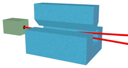
Stern-Gerlach device. An oven (left, green) produces a beam of silver atoms (red) that passes between two powerful magnets (blue), which splits the beam into two distinct beams of atoms with “spin-up” and “spin-down” eigenstates relative to the vertical axis. To measure the horizontal (or any other) axis, the device is physically rotated to the desired angle.

This result comes from the Stern-Gerlach experiment. The assumption was that the magnetic field would result in a fan-like spray of silver atoms with various spin values reacting to the magnetic field. Instead, the atoms formed two distinct streams, one deflected up, the other down.

Unlike energy or momentum, which can have many quantum values, spin is a strictly binary property. That is why it’s one of the simpler quantum systems. (At least when talking about spin 1/2 particles.)

These spin experiments demonstrate an important property of quantum states: they can be non-commutative — the order of measurements matters and, further, that measurements are not compatible with each other.

The following series of experiments illustrates this key difference between the classical and the quantum worlds.

§ §

Figure 1. Spin test, Z-axis.

First, we need to understand a basic spin measurement.

Popular accounts and lectures sometimes invoke a sort of magic box that produces objects or tests properties such as hard/soft or black/white. I’m going to skip that (for now) and jump right to a magic box that measures spin.

Not so magic, really, because Stern-Gerlach devices are real, and work as described. All these experiments have actually been performed, and they confirm quantum predictions.

Figure 1 shows a single spin test. Particles enter the box from the left and exit right or down depending on their measured spin (spin-up or spin-down, respectively). The “Z” indicates this box measures the Z-axis. A reflector diverts the spin-down stream to the right (you’ll see why below).

The 100% on the left indicates that all particles enter the box. The wheel shape below it indicates the particles have unknown, and presumably mixed, spins — we assume an even distribution of spins.

We’re skipping past the notion that particles that have never been measured even have a distinct spin. Quantum mechanics suggests they do not; philosophical realism suggests they must have. (The jury is hung on this one; court is adjourned.)

Given the presumed even distribution (or that spin is undetermined), over time we would expect an equal mix of spin-up and spin-down measurements. That’s exactly what we find: 50% turn out to be spin-up; 50% turn out to be spin-down. (The blue numbers on the right reflect this fact.)

Note that we can set the box to measure any angle, and we always get a 50/50 mix of spin-up and spin-down relative to the chosen axis.

There are a number of ways spin states are represented mathematically. All are just different ways of notating the same thing depending on what the author wants to say.

For the spin-up state:

$|up\rangle=|{+}\rangle=|{0}\rangle=|Z_{+}\rangle=\begin{bmatrix}{1}\\{0}\end{bmatrix}$

And for the spin-down state:

$|down\rangle=|{-}\rangle=|{1}\rangle=|Z_{-}\rangle=\begin{bmatrix}{0}\\{1}\end{bmatrix}$

The first version is a casual, but evocative, notation. The second and third are the most common from what I’ve seen (I’ll be using the third in this post). The fourth is explicit about which axis is involved, which can be helpful when dealing with multiple axes in one equation. The fifth is the column vector for the eigenstate actually used in calculations.

Remember that any measurement of a quantum system involves eigenstates (aka eigenvectors) representing the possible outcomes. Both the spin-up and spin-down results are such eigenstates. As mentioned above, they are the only possible outcomes of a measurement on a spin 1/2 particle.

We view a particle with an unknown spin as a superposition of the two possible spin eigenstates. We can write this as:

$\psi=\alpha\!\mid\!{0}\rangle+\beta\!\mid\!{1}\rangle$

Where α (alpha) and ß (beta) are (complex number) coefficients representing the (normalized) probability of getting that measurement. For a given particle with unknown spin, we have no way to know these coefficients.

However, in an even distribution of spins and many measurements, we know the outcomes divide equally, so we know that in the general case we have:

$\psi=\frac{1}{\sqrt{2}}\!\mid\!{0}\rangle+\frac{1}{\sqrt{2}}\!\mid\!{1}\rangle$

The actual probability is the norm squared of these coefficients, and:

$|\frac{1}{\sqrt{2}}|^2=\frac{1}{2},\;\;\;\frac{1}{2}+\frac{1}{2}=1$

A measurement always has some outcome, so the probabilities always must sum to 1.

This all applies to any axis at any angle, but traditionally the Z-axis, the vertical axis, is the basis of our treatment. As such, we assign the |0〉 (“ket zero”) eigenstate to a spin-up measurement on that axis and the |1〉 (“ket 1”) state to the spin-down measurement.

We call this the {|0〉, |1〉} eigenbasis, and this basis spans all possible spin states, including those on other axes.

This is an important point. Particles with spin 1/2 have three orthogonal axis, X, Y, and Z. One might think we also need an eigenbasis for the other two axes. We do not. The {|0〉, |1〉} basis spans all possible spin states.

We represent those other states as superposition of the basis states. For the X-axis:

$\mid\!{+}\rangle=\frac{\mid{0}\rangle\;+\;\mid{1}\rangle}{\sqrt{2}},\;\;\mid\!{-}\rangle=\frac{\mid{0}\rangle\;-\;\mid{1}\rangle}{\sqrt{2}}$

And for the Y-axis:

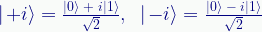
$\mid\!{+i}\rangle=\frac{\mid{0}\rangle\;+\;{i}\mid{1}\rangle}{\sqrt{2}},\;\;\mid\!{-i}\rangle=\frac{\mid{0}\rangle\;-\;{i}\mid{1}\rangle}{\sqrt{2}}$

Note the minus signs in the spin-down states.

Our two eigenstates, the eigenbasis, give us a complete description of the possible spin states.

Another important point: After a measurement we know the spin state, and the state vector has jumped (“collapsed”) to that state. If, for instance, we had measured spin-up, the quantum state is now just:

$\psi=\mid\!{0}\rangle$

Further measurements return the same result with 100% probability.

§ §

Which brings us to the next experiment. This involves three Z-boxes, all performing the same test of spin on the Z-axis:

Figure 2. The blue percentages show how many particles exit a box given all that enter. The red percentages show total percentages of particles at the end of the experiment.

As you see, the outputs from the first test are funneled to second tests which repeat the Z-axis test (the reflector redirects the streams for the sake of the diagrams but wouldn’t exist in a real experiment because it would affect the particle spins).

This experiment shows how the first test puts the particles into known eigenstates such that further immediate tests on the particle have a 100% chance of giving the same results. (Unlike the first test where it was 50% each.)

We see a similar thing with photons and polarizing filters. A photon that does pass through a vertical polarizer is now vertically polarized and passes through a second vertical filter with 100% probability.

This, so far, seems almost classical behavior, as long as we accept that we’ve changed the wave-function of the particles after the first test. (The second tests make no change.) Given that change in the first test, the behavior in the second tests is what we’d expect.

§ §

Now let’s try measuring a different axis in the second test. We’ll measure the X-axis second:

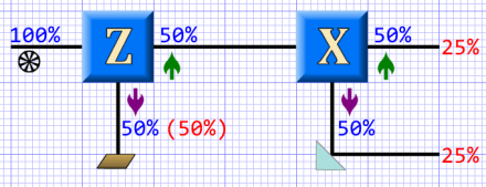
Figure 3. Measuring the X-axis after measuring the Z-axis. (We’re discarding the particles with spin-down in the first test. If sent through a X-axis test, that test would also produce 50/50 results.)

With spin, orthogonal axes are not correlated, and since we know the value of the Z-axis measurement, we can know nothing about the state of spin on the X-axis (or the Y-axis).

It’s not merely our ignorance; the spin state on the X-axis is undetermined. Because the particle is now in a known eigenstate, |0〉 on the Z-axis, spin on orthogonal axes is an equal superposition of possible results on those axes. As such, we expect 50/50 results over multiple tests.

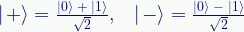
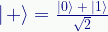
As shown above, the X-axis measurement implies another basis, usually written as {|+〉, |-〉}, but defined in terms of the eigenbasis, {|0〉, |1〉}:

$\mid\!+\rangle=\frac{\mid{0}\rangle\;+\;\mid{1}\rangle}{\sqrt{2}},\;\;\;\mid\!-\rangle=\frac{\mid{0}\rangle\;-\;\mid{1}\rangle}{\sqrt{2}}$

Note that we’re seeing quantum behavior in the sense that knowing the spin state of the Z-axis makes the spin state of the X-axis undetermined. These orthogonal measurements are incompatible.

The next experiment drives home this point.

§ §

This experiment starts off the same way as the previous one, but adds a third test, a second Z-axis test. Above we saw that repeating a test of the same axis gave the same result. But here…

Figure 4. Three tests, Z-X-Z. (Particles from the first tests discarded.)

We see that the third test has a 50/50 split of particles! The second test erased the first result. This is implicit in the definition of the |+〉 state:

$\mid\!+\rangle=\frac{\mid{0}\rangle\;+\;\mid{1}\rangle}{\sqrt{2}}$

That state is a superposition of the |0〉 and |1〉 states, as it was before the first test.

§ §

This all just scratches the surface. The main point is that knowing the spin state on a given axis means the spin state of the other orthogonal axes is a fully undetermined superposition of possible outcomes. The probability is 50/50.

If we measure a non-orthogonal axis, we see a correlation that depends on the angle. The superposition then looks like:

$\psi=\cos^2\theta\mid\!{0}\rangle+\sin^2\theta\mid\!{1}\rangle$

Where θ (theta) is the angle relative to |0〉. The closer that angle, the higher the probability of getting the |0〉 result.

Lastly, recognize that, not only are spin measurements not compatible — knowing spin on a measured axis erases our knowledge of all other axes — but also non-commutative. The order of measurements obviously matters.

This is a key aspect (some say the key aspect) of the quantum world. It’s embodied in the Heisenberg Uncertainty Principle.

§ §

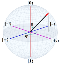
Next time I’ll talk about quantum states and explain that blue sphere (the Bloch sphere) that’s been the header image for this post series.

Stay spinning, my friends! Go forth and spread beauty and light.

∇

About Wyrd Smythe

The canonical fool on the hill watching the sunset and the rotation of the planet and thinking what he imagines are large thoughts. View all posts by Wyrd Smythe

This entry was posted on Monday, March 8th, 2021 at 12:00 pm and tagged with QM101, quantum mechanics, quantum spin and posted in Math, Physics. You can follow any responses to this entry through the RSS 2.0 feed.

36 responses to “QM 101: Quantum Spin”

Wyrd Smythe
March 8th, 2021 at 12:12 pm

An interesting aspect to the Stern-Gerlach experiment, a question I’ve had about it and recently saw answered, is that — until the silver atoms actually strike a surface and make an “image” (of splattered silver atoms on, usually, a glass surface) under the MWI the beams are in superposition.

So, with regard to the last test, the first test branches into two “worlds” and a second stage test then branches those into two (four total) and a third stage branches yet again (eight total). So (under the MWI), if a single silver atom were tested in three stages, eight different versions of the experiment exist, one for each of the possible outcomes.

What’s not clear to me is whether the test with three Z boxes results in only two branches or four. I don’t know if the second stage — with its fully determined result — causes a branch.

Reply
- SelfAwarePatterns
  March 9th, 2021 at 11:13 am
  
  I think this is one of those zen things Aaronson was talking about.
  
  If under Everett we view a branch as portions of the wavefunction diverging from each other, then I don’t think the second stage causes a branch.
  
  Of course it’s still a measurement, meaning decoherence, the outcome of a quantum event is still amplified into the environment and entangled with it, so we could still view that as the world splitting into additional worlds, but they’d be identical. If we have multiple worlds identical to each other (at least macroscopically), are they really separate worlds?
  
  Or if we take the view we discussed on the other thread that it’s all preexisting worlds, then it’s a situation where all the worlds where the second stage took place didn’t diverge from each other as a result of the measurement.
  
  It seems like the important thing is the divergence, or lack thereof.
  
  At least, that’s my current answer. 🙂
  
  Reply
  - Wyrd Smythe
    March 9th, 2021 at 11:24 am
    
    It does boil down to exactly what causes a branch, doesn’t it. It’s one of many things I keep hoping an expert who has really studied this would clear up. I don’t find “dealer’s choice” very satisfying.
Wyrd Smythe
March 8th, 2021 at 12:13 pm

This $%&# Dell XPS 15 laptop is driving me crazy with it’s intermittent “DNS? What DNS?” issue that comes and goes. This morning it’s been really plaguing me. A pox on Dell!

(It’s not that my internet is the problem, the laptop can’t even connect to the explicit IP (*.*.0.1) of my router. No clue if the problem is the WiFi or Windows itself. I suspect the WiFi, though.)

Reply
- Wyrd Smythe
  March 8th, 2021 at 2:13 pm
  
  God, it’s bad today, this damn laptop. Constantly losing the DNS. I wish I knew why or what to do. 😦 😦 😦
  
  Reply
- Wyrd Smythe
  March 11th, 2021 at 10:43 am
  
  Huh, interesting. Back when these laptop network issues started I wrote a Python app, netprobe, that does a loop of making the same http request every T seconds for N many times. Usually I set T to 90 seconds and N to some large number to keep it going all day.
  
  IIRC I posted some charts showing the failure rates. At the time I was trying to zero down on whether time of day was a factor. It didn’t appear to be. If anything, the data was characterized by times that didn’t seem to have problems. Most of the day did.
  
  Yesterday I dug out the app and set T to 60 seconds, and to my astonishment, that seems to keep the computer connected. I haven’t had a DNS error while it was running.
  
  As another data point, when N expired last night while I was watching TV, and then I came to use the computer later, there was a DNS issue at first. (These DNS issues seem to self-correct after first telling me it can’t.)
  
  So new theory. (Or rather, one of many theories now seems to maybe be the case.) I think the network card is going to sleep and not waking up appropriately when a network request is made.
  
  If that’s the case, maybe replacing the network component, if that’s possible, would fix it, but if all I have to do is have Python ping my router every 60 seconds, that’s an acceptable “fix” for now.
  
  I’ll surely be a whole lot less frustrated with the situation!
  
  Reply
  - Michael
    March 11th, 2021 at 7:40 pm
    
    I felt great joy when I read this, Wyrd.
  - Wyrd Smythe
    March 11th, 2021 at 9:37 pm
    
    😀 And for about two days now, my “fix” seems to be working.
    
    I just did my income taxes and I obviously need to do something about my withholding. I had to pay nearly five grand, so I’m not in a happy camper mode right now. But at least they’re done. One of my least favorite parts of the year.
  - Wyrd Smythe
    March 25th, 2021 at 8:53 am
    
    Heh. My workaround has been working great, and I’ve been thinking I should try not running it for a while to see if it’s really the reason I haven’t experienced the error. (There was a big Windows update last week, and I thought it might have improved things.)
    
    But this morning, I started doing something without starting my netprobe app, and, bingo, had the “DNS? What DNS?” problem right away. (Damned Dell.)
    
    So, yeah, it really looks like making a network request — even just to my router — every 60 seconds does the trick. At this point I’m assuming the network card goes to sleep and has trouble waking up.
    
    Have I mentioned how much I hate this fucking Dell laptop?
Wyrd Smythe
March 8th, 2021 at 2:09 pm

It might be worth mentioning that, in terms of how we talk about states off the basis axis (Z, in this case), the |X+⟩ and |X-⟩ states, as well as the |Y+⟩ and |Y+⟩ states, are not (as I understand it) actually eigenstates. Our measurement is, in this treatment, strictly on the Z-axis.

If we rotate the S-G device to measure some other axis, our measurement eigenstates are, as always, |0⟩ and |1⟩, and it is axes different from whatever one we selected that are now described in terms of superpositions of these eigenstates.

The point is that there are only ever two eigenstates, |0⟩ and |1⟩ —, which is all that can be tested at any given point. All other possible states we could choose to measure are described in terms of those.

Reply
- Wyrd Smythe
  March 8th, 2021 at 2:12 pm
  
  Side note: I think it’s high time I stopped italicizing eigenthings.
  
  Reply
Michael
March 8th, 2021 at 7:02 pm

Very interesting, Wyrd. I’m reading posts I’ve missed backwards, but you wrote very clearly and I don’t feel I’ve misunderstood anything even if I can only vaguely describe what an operator is. (I’ll go back and read, so no need to take your time to explain it below.)

But a couple questions:

1. A spin 1/2 particle can have spins on three independent axes that are not correlated. If we know the spin in the Z direction is up or down, anything is possible for X or Y. So which is the Stern-Gerlach experiment measuring? Or does it have to do with the physical orientation of the magnets with respect to the local gravitational field and the direction of the particles’ travel? Meaning, the orientation of gravity defines the Z axis? And the direction of particle travel defines the X and Y (one being parallel to the direction of travel and the other being perpendicular?) Or is gravity wholly unrelated and the particle’s local coordinate system defines everything? You see what I’m asking by now I’m sure.

2. Is there some kind of right-hand or left-hand rule about this quantum spin? Or that’s just nonsense to talk about? Meaning, if we’re conducting a Z-axis test of spin, does the up result mean it’s spinning clockwise as we look up? And a down result mean it’s spinning that way looking down? I know you said there’s not anything actually spinning, but… I couldn’t help myself. [sheepish grin]

3. What is spin, anyway?

Michael

Reply
- Wyrd Smythe
  March 8th, 2021 at 9:33 pm
  
  I’m glad you found it interesting! Keeping mind we’re approaching the edges of my firm understanding, your questions in reverse order…
  
  “What is spin, anyway?”
  
  😀 No one really knows! Particles in a strong magnetic field deflect from their straight path because they have a magnetic moment that, quantizing aside, acts very much like a spinning magnet.
  
  “Is there some kind of right-hand or left-hand rule about this quantum spin?”
  
  It doesn’t seem to come up in most discussions of spin that I’ve seen, although in particle physics there is both the notion of chirality and helicity, which do have some connection with spin. (Some particles are “left-handed” and “right-handed” for example.)
  
  But, for instance, the Wiki spin article doesn’t mention either in the text, but does list both in the “See also” section.
  
  FWIW, photons (spin 0 particles) have two spin states, circular left and circular right. Depending on how those are superposed, light is one, the other, or a combination that makes the polarization vertical, horizontal, or elliptical. (Polarization of light is photon spin.)
  
  Photon polarization is still a topic I’m exploring. See the Wiki Polarization article if you want to dig into it.
  
  “Meaning, if we’re conducting a Z-axis test of spin, does the up result mean it’s spinning clockwise as we look up? And a down result mean it’s spinning that way looking down?”
  
  I don’t believe it works that way, mostly based on that direction is never mentioned in the treatments of spin I’ve seen. But maybe, if one really digs into the weeks… [shrug]
  
  Your first question is so substantial I think I’ll tackle it separately so my reply doesn’t become a post in itself!
  
  Reply
- Wyrd Smythe
  March 8th, 2021 at 9:55 pm
  
  “So which is the Stern-Gerlach experiment measuring?”
  
  The convention is that the Z-axis is vertical (i.e. aligned with the gravity gradient), but that is purely a convention. The S-G device deflects the beams “up” or “down” with respect to the device (as shown in the diagram).
  
  If we want to measure the horizontal axis, the device must be rotated 90° — or to whatever angle we wish to measure. The spin measurement depends only the orientation of the magnets. The magnetic moment of the particle interacts with the magnetic field, which causes the deflection.
  
  Again conventionally, the X-axis is taken as the horizontal axis, perpendicular to the particle’s motion. The Z-axis, likewise, is also perpendicular to the direction of travel.
  
  The Y-axis is the direction of travel, and I’m not sure how they measure that. The Wiki article for the Stern-Gerlach experiment only discusses the Z and X axes. (It does have a treatment of the experiments I covered in the post.)
  
  As I replied to your comment on the eigenvectors post, there are three canonical spin operators for spin 1/2 systems, one for each axis. They’re called the Pauli matrices, usually called sigma X, Y, and Z.
  
  For the Z-axis:
  
  $\sigma_z=\frac{\hbar}{2}\begin{bmatrix}{1}&{0}\\{0}&{-1}\end{bmatrix}$
  
  For the X-axis:
  
  $\sigma_x=\frac{\hbar}{2}\begin{bmatrix}{0}&{1}\\{1}&{0}\end{bmatrix}$
  
  For the Y-axis:
  
  $\sigma_y=\frac{\hbar}{2}\begin{bmatrix}{0}&{-i}\\{i}&{0}\end{bmatrix}$
  
  And you’ll note the last one does have complex values.
  
  Reply
Wyrd Smythe
March 8th, 2021 at 10:50 pm

A little fun with quantum math…

In terms of those Pauli matrices, we can derive the eigenvalues using the equation (see this comment for other examples):

$p(\lambda)=\det(M-\lambda\mathbb{I})=0$

For the Z-axis:

$\det\big(\begin{bmatrix}{\frac{\hbar}{2}}&{0}\\{0}&{\frac{-\hbar}{2}}\end{bmatrix}-\begin{bmatrix}{\lambda}&{0}\\{0}&{\lambda}\end{bmatrix}\big)=0$

Doing the subtraction:

$\det\big(\begin{bmatrix}{\frac{\hbar}{2}-\lambda}&{0}\\{0}&{\frac{-\hbar}{2}-\lambda}\end{bmatrix}\big)=0$

Which gives us:

$(\frac{\hbar}{2}-\lambda)(\frac{-\hbar}{2}-\lambda)=0$

So λ obviously has to be plus and minus hbar-over-two.

For the X-axis:

$\det\big(\begin{bmatrix}{0}&{\frac{\hbar}{2}}\\{\frac{\hbar}{2}}&{0}\end{bmatrix}-\begin{bmatrix}{\lambda}&{0}\\{0}&{\lambda}\end{bmatrix}\big)=0$

Doing the subtraction:

$\det\big(\begin{bmatrix}{-\lambda}&{\frac{\hbar}{2}}\\{\frac{\hbar}{2}}&{-\lambda}\end{bmatrix}\big)=0$

Which gives us:

$\lambda^2-(\frac{\hbar}{2})^2=0$

Which we can factor:

$(\lambda+\frac{\hbar}{2})(\lambda-\frac{\hbar}{2})=0$

And again λ has to be plus and minus hbar-over-two.

Finally, for the Y-axis:

$\det\big(\begin{bmatrix}{0}&{\frac{-{i}\hbar}{2}}\\{\frac{{i}\hbar}{2}}&{0}\end{bmatrix}-\begin{bmatrix}{\lambda}&{0}\\{0}&{\lambda}\end{bmatrix}\big)=0$

Doing the subtraction:

$\det\big(\begin{bmatrix}{-\lambda}&{\frac{-{i}\hbar}{2}}\\{\frac{{i}\hbar}{2}}&{-\lambda}\end{bmatrix}\big)=0$

Which gives us:

$\lambda^2-(\frac{{i}\hbar}{2})(\frac{-{i}\hbar}{2})=0$

Which is:

$\lambda^2-\frac{\hbar^2}{4}=0$

Which factors the same way as for the X-axis, and again λ is plus and minus hbar-over-two.

Reply
Wyrd Smythe
March 9th, 2021 at 12:18 am

To derive the eigenvectors, we use the equation:

$(M-\lambda_i\mathbb{I})v=0$

For the Z-axis, for +hbar/2:

$\big(\begin{bmatrix}{\frac{\hbar}{2}}&{0}\\{0}&{\frac{-\hbar}{2}}\end{bmatrix}-\begin{bmatrix}{\frac{\hbar}{2}}&{0}\\{0}&{\frac{\hbar}{2}}\end{bmatrix}\big)v=0$

Which is:

$\begin{bmatrix}{0}&{0}\\{0}&{\hbar}\end{bmatrix}{v}=0$

Which means v can be:

$\begin{bmatrix}{0}&{0}\\{0}&{\hbar}\end{bmatrix}\begin{bmatrix}{x}\\{0}\end{bmatrix}=0$

So the characteristic vector is (1,0), also known as the |0⟩, the spin up result.

For the Z-axis, for -hbar/2:

$\big(\begin{bmatrix}{\frac{\hbar}{2}}&{0}\\{0}&{\frac{-\hbar}{2}}\end{bmatrix}-\begin{bmatrix}{\frac{-\hbar}{2}}&{0}\\{0}&{\frac{-\hbar}{2}}\end{bmatrix}\big)v=0$

Which is:

$\begin{bmatrix}{\hbar}&{0}\\{0}&{0}\end{bmatrix}{v}=0$

Which means v can be:

$\begin{bmatrix}{0}&{0}\\{0}&{\hbar}\end{bmatrix}\begin{bmatrix}{0}\\{y}\end{bmatrix}=0$

So the characteristic vector is (0,1), also known as |1⟩, the spin down result.

For the X-axis, for +hbar/2:

$\big(\begin{bmatrix}{0}&{\frac{\hbar}{2}}\\{\frac{\hbar}{2}}&{0}\end{bmatrix}-\begin{bmatrix}{\frac{\hbar}{2}}&{0}\\{0}&{\frac{\hbar}{2}}\end{bmatrix}\big)v=0$

Which is:

$\begin{bmatrix}{\frac{-\hbar}{2}}&{\frac{\hbar}{2}}\\{\frac{\hbar}{2}}&{\frac{-\hbar}{2}}\end{bmatrix}{v}=0$

Which means v can be:

$\begin{bmatrix}{\frac{-\hbar}{2}}&{\frac{\hbar}{2}}\\{\frac{\hbar}{2}}&{\frac{-\hbar}{2}}\end{bmatrix}\begin{bmatrix}{x}\\{x}\end{bmatrix}=0$

So the characteristic vector is (1,1), or as a normalized vector:

$\begin{bmatrix}\frac{1}{\sqrt{2}}\\\frac{1}{\sqrt{2}}\end{bmatrix}$

For the X-axis, for -hbar/2:

$\big(\begin{bmatrix}{0}&{\frac{\hbar}{2}}\\{\frac{\hbar}{2}}&{0}\end{bmatrix}-\begin{bmatrix}{\frac{-\hbar}{2}}&{0}\\{0}&{\frac{-\hbar}{2}}\end{bmatrix}\big)v=0$

Which is:

$\begin{bmatrix}{\frac{\hbar}{2}}&{\frac{\hbar}{2}}\\{\frac{\hbar}{2}}&{\frac{\hbar}{2}}\end{bmatrix}{v}=0$

Which means v can be:

$\begin{bmatrix}{\frac{\hbar}{2}}&{\frac{\hbar}{2}}\\{\frac{\hbar}{2}}&{\frac{\hbar}{2}}\end{bmatrix}\begin{bmatrix}{x}\\{-x}\end{bmatrix}=0$

So the characteristic vector is (1,-1), or as a normalized vector:

$\begin{bmatrix}\frac{1}{\sqrt{2}}\\\frac{-1}{\sqrt{2}}\end{bmatrix}$

Note that the |+⟩ superposition for the X-axis is:

$\frac{1}{\sqrt{2}}(|0\rangle\!+\!|1\rangle)=\frac{1}{\sqrt{2}}\big(\!\begin{bmatrix}{1}\\{0}\end{bmatrix}\!+\!\begin{bmatrix}{0}\\{1}\end{bmatrix}\big)\!=\!\begin{bmatrix}{\frac{1}{\sqrt{2}}}\\{\frac{1}{\sqrt{2}}}\end{bmatrix}$

And the |-⟩ superposition for the X-axis is:

$\frac{1}{\sqrt{2}}(|0\rangle\!-\!|1\rangle)=\frac{1}{\sqrt{2}}\big(\!\begin{bmatrix}{1}\\{0}\end{bmatrix}\!-\!\begin{bmatrix}{0}\\{1}\end{bmatrix}\big)\!=\!\begin{bmatrix}{\frac{1}{\sqrt{2}}}\\{\frac{-1}{\sqrt{2}}}\end{bmatrix}$

For the Y-axis,… I’ll leave that as an exercise for the dedicated reader! 🙂

Reply
Wyrd Smythe
March 10th, 2021 at 6:02 pm

Okay, now that I’ve had a chance to recover from all that LaTeX, for completeness, let’s do the Y-axis eigenvectors.

For the Y-axis, +hbar/2:

$\displaystyle\big(\begin{bmatrix}{0}&{\frac{{-i}\hbar}{2}}\\{\frac{{i}\hbar}{2}}&{0}\end{bmatrix}-\begin{bmatrix}{\frac{\hbar}{2}}&{0}\\{0}&{\frac{\hbar}{2}}\end{bmatrix}\big)v=0$

Which is:

$\begin{bmatrix}{\frac{-\hbar}{2}}&{\frac{{-i}\hbar}{2}}\\{\frac{{i}\hbar}{2}}&{\frac{-\hbar}{2}}\end{bmatrix}{v}=0$

Which means v can be:

$\begin{bmatrix}{\frac{-\hbar}{2}}&{\frac{{-i}\hbar}{2}}\\{\frac{{i}\hbar}{2}}&{\frac{-\hbar}{2}}\end{bmatrix}\!\!\begin{bmatrix}{1}\\{i}\end{bmatrix}=\begin{bmatrix}{\frac{-\hbar}{2}}+{\frac{{-i}^2\hbar}{2}}\\{\frac{{i}\hbar}{2}}+{\frac{{-i}\hbar}{2}}\end{bmatrix}=\begin{bmatrix}{\frac{-\hbar}{2}}+{\frac{\hbar}{2}}\\{\frac{{i}\hbar}{2}}+{\frac{{-i}\hbar}{2}}\end{bmatrix}=\begin{bmatrix}0\\0\end{bmatrix}$

So the eigenvector is (1,i), or as a normalized vector:

$\begin{bmatrix}\frac{1}{\sqrt{2}}\\\frac{i}{\sqrt{2}}\end{bmatrix}$

For the Y-axis, -hbar/2:

$\big(\begin{bmatrix}{0}&{\frac{{-i}\hbar}{2}}\\{\frac{{i}\hbar}{2}}&{0}\end{bmatrix}-\begin{bmatrix}{\frac{-\hbar}{2}}&{0}\\{0}&{\frac{-\hbar}{2}}\end{bmatrix}\big)v=0$

Which is:

$\begin{bmatrix}{\frac{\hbar}{2}}&{\frac{{-i}\hbar}{2}}\\{\frac{{i}\hbar}{2}}&{\frac{\hbar}{2}}\end{bmatrix}{v}=0$

Which means v can be:

$\begin{bmatrix}{\frac{\hbar}{2}}&{\frac{{-i}\hbar}{2}}\\{\frac{{i}\hbar}{2}}&{\frac{\hbar}{2}}\end{bmatrix}\!\!\begin{bmatrix}{1}\\{-i}\end{bmatrix}=\begin{bmatrix}{\frac{\hbar}{2}}+{\frac{{i}^2\hbar}{2}}\\{\frac{{i}\hbar}{2}}+{\frac{{-i}\hbar}{2}}\end{bmatrix}=\begin{bmatrix}{\frac{\hbar}{2}}+{\frac{-\hbar}{2}}\\{\frac{{i}\hbar}{2}}+{\frac{{-i}\hbar}{2}}\end{bmatrix}=\begin{bmatrix}0\\0\end{bmatrix}$

So the eigenvector is (1,-i), or as a normalized vector:

$\begin{bmatrix}\frac{1}{\sqrt{2}}\\\frac{-i}{\sqrt{2}}\end{bmatrix}$

Which all does get a bit math-y having to deal with i.

Note that the |+i⟩ superposition for the Y-axis is:

$\frac{1}{\sqrt{2}}(|0\rangle\!+\!{i}|1\rangle)=\frac{1}{\sqrt{2}}\big(\!\begin{bmatrix}{1}\\{0}\end{bmatrix}\!+\!{i}\begin{bmatrix}{0}\\{1}\end{bmatrix}\big)\!=\!\begin{bmatrix}{\frac{1}{\sqrt{2}}}\\{\frac{i}{\sqrt{2}}}\end{bmatrix}$

And the |-i⟩ superposition for the Y-axis is:

$\frac{1}{\sqrt{2}}(|0\rangle\!-\!{i}|1\rangle)=\frac{1}{\sqrt{2}}\big(\!\begin{bmatrix}{1}\\{0}\end{bmatrix}\!-\!{i}\begin{bmatrix}{0}\\{1}\end{bmatrix}\big)\!=\!\begin{bmatrix}{\frac{1}{\sqrt{2}}}\\{\frac{-i}{\sqrt{2}}}\end{bmatrix}$

So once again the eigenvectors of the spin operators are the canonical superpositions of the spin states.

Reply
Wyrd Smythe
March 10th, 2021 at 6:18 pm

The point is that each of the three spin operators has its own pair of eigenvectors, which are the canonical superpositions, and in all three cases the eigenvalues are plus and minus hbar-over-two.

Reply
Wyrd Smythe
March 10th, 2021 at 6:50 pm

As a check of our eigenvalues and eigenvectors, recall from the Eigen Whats? post that the trace of a matrix is the sum of eigenvalues:

$\displaystyle\mathsf{trace}(M)=\sum^{2}_{i}\lambda_i=\lambda_1+\lambda_2$

And the determinant is their product:

$\displaystyle\mathsf{det}(M)=\prod^{2}_{i}\lambda_i=\lambda_1\times\lambda_2$

We (think we) know our eigenvalues here are:

$\lambda_1=\frac{+\hbar}{2},\;\;\;\lambda_2=\frac{-\hbar}{2}$

Our spin operator matrices are:

$\sigma_z\!=\!\begin{bmatrix}{\frac{\hbar}{2}}&{0}\\{0}&{\frac{-\hbar}{2}}\end{bmatrix},\;\sigma_x\!=\!\begin{bmatrix}{0}&{\frac{\hbar}{2}}\\{\frac{\hbar}{2}}&{0}\end{bmatrix},\;\sigma_y\!=\!\begin{bmatrix}{0}&{\frac{{-i}\hbar}{2}}\\{\frac{{i}\hbar}{2}}&{0}\end{bmatrix}$

So:

$\mathsf{trace}(\sigma_z)=\frac{+\hbar}{2}+\frac{-\hbar}{2}=0$

Both the σ_x and σ_y matrices have zeros on their main diagonals, so:

$\mathsf{trace}(\sigma_x)\!=0\!+\!0\!=\!0,\;\;\;\mathsf{trace}(\sigma_y)\!=0\!+\!0\!=\!0$

Our eigenvalues obviously sum to zero, so we expect the trace to be zero, and it is.

The product of the eigenvalues is:

$\frac{+\hbar}{2}\times\frac{-\hbar}{2}=\frac{-\hbar^2}{4}$

The determinant of our matrices is:

$\mathsf{det}(\sigma_z)=\big(\frac{\hbar}{2}\!\times\!\frac{-\hbar}{2}\big)-(0\times\!0)=\frac{-\hbar^2}{4}$

And:

$\mathsf{det}(\sigma_x)=(0\times\!0)-\big(\frac{\hbar}{2}\!\times\!\frac{\hbar}{2}\big)=\frac{-\hbar^2}{4}$

And:

$\mathsf{det}(\sigma_y)=(0\times\!0)-\big(\frac{{i}\hbar}{2}\!\times\!\frac{{-i}\hbar}{2}\big)=\frac{-\hbar^2}{4}$

So it all checks out.

Reply
QM 101: Bloch Sphere | Logos con carne
March 15th, 2021 at 7:28 am

[…] is quantum spin, which I wrote about last time. The sphere idea dates back to 1892 when Henri Poincaré defined the Poincaré sphere to describe […]

Reply
QM101: Bra-Ket Notation | Logos con carne
March 22nd, 2021 at 7:31 am

[…] a ket denotes a quantum state. For example, in two-level quantum systems (see: Bloch Sphere and Quantum Spin) we have the canonical […]

Reply
Wyrd Smythe
May 25th, 2021 at 12:54 pm

Here’s a nice video about the Stern-Gerlach experiment:

Reply
Wyrd Smythe
July 7th, 2021 at 9:36 pm

Here’s a really good video from PBS SpaceTime:

Reply
Sai Sundar S
July 29th, 2021 at 12:47 pm

Nice article explaining the matrix approach of states it’s superposition. Practicing matrix approach helps me to study various gates involved in Q computing and I am on the path of learning it The notes on raising operator and lowering operators also I had prepared in terms of matrix It is really a fantastic writing Thank you.

Reply
- Wyrd Smythe
  July 29th, 2021 at 12:50 pm
  
  Thanks! I’m glad it was useful for you!
  
  Reply
Sai Sundar S
July 29th, 2021 at 12:50 pm

The Blotch sphere also clearly explaining ket 0 and 1

Reply
- Wyrd Smythe
  July 29th, 2021 at 12:51 pm
  
  Yep!
  
  Reply
  - Sai Sundar S
    July 29th, 2021 at 12:56 pm
    
    Frankly speaking I could not understand the post in the site
  - Wyrd Smythe
    August 1st, 2021 at 10:04 am
    
    One can always ask questions about points that aren’t clear, but it looks like another post here already answered them?
Sai Sundar S
July 29th, 2021 at 12:58 pm

Ok now I had seen the article on blotch sphere Thank you I got it

Reply
- Wyrd Smythe
  August 1st, 2021 at 10:07 am
  
  So the other post answered your questions? Great! This and that post are part of a series about QM.
  
  Reply
Sai Sundar S
July 29th, 2021 at 12:59 pm

Pauli matrix x y and z all are clearly explained and eigen also Really fantastic to see this post

Reply
- Wyrd Smythe
  August 1st, 2021 at 10:08 am
  
  Thanks, again! Glad you enjoyed it!
  
  Reply
QM 101: Photon Spin | Logos con carne
August 25th, 2021 at 7:07 am

[…] in this QM-101 series I posted about quantum spin. That post looked at spin 1/2 particles, such as electrons (and silver atoms). This post looks at […]

Reply
BB #75: Gloves and Shoes | Logos con carne
August 27th, 2021 at 7:28 am

[…] When I wrote about quantum spin I explicitly stayed away from “magic” boxes and discussed Stern-Gerlach devices, but a classical analogy seems to require them. My magic box contains either one glove or one shoe, depending on whether one opens the top (glove) or side (shoe). […]

Reply
2022: I Hardly Knew Ya | Logos con carne
January 14th, 2023 at 3:09 pm

[…] QM 101: Quantum Spin (2021, 112) […]

Reply