QM 101: Linear Transforms

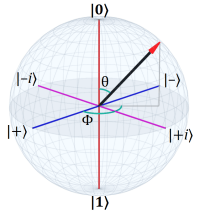
Last time I set the stage, the mathematical location for quantum mechanics, a complex vector space (Hilbert space) where the vectors represent quantum states. (A wave-function defines where the vector is in the space, but that’s a future topic.)

The next mile marker in the journey is the idea of a transformation of that space using operators. The topic is big enough to take two posts to cover in reasonable detail.

This first post introduces the idea of (linear) transformations.

I mentioned in the Introduction that, despite the unfamiliar name, linear transformations — using linear algebra — are just a cool kind of geometry.

As with many forms of geometry, linear algebra generalizes to any number of dimensions, but (as with many forms of geometry) we’ll explore it in two dimensions to build the necessary intuitions.

So we will assume a 2D Euclidean space that we’ll view as vector space. (See previous post for details.)

Every point in the space has an associated arrow (a vector) with its tail at the origin and its tip at the point. These vectors give each point a magnitude, eta (η), and an angle, theta (θ).

Additionally, we multiply the Y-axis by the imaginary unit, i, to create the 2D complex plane. This lets us leverage the following identities:

The third form, the exponential, is especially helpful in wave mechanics in general and in quantum mechanics in particular. We’ll explore that in more detail in future posts. For now we start simply…

§ §

A transformation in this space is a function (or something we treat as one) that takes a vector from the space and returns a new vector. We say a transformation maps vectors to new positions in the space.

The simplest transformation is to do nothing at all. For now, we’ll call this the Null transformation. It maps all vectors onto themselves. (Think of it as multiplying by one.) We’ll use notation that looks like this:

This defines transformation T, which takes complex number z as input. In this case the transformation is defined as simply the input vector, z.

Figure 1. The space before (left) and after (right) the Null transform.

A transform map need not be bijective; it can be non-injective and/or non-surjective. The domain (the input) is all vectors, but the codomain (the output) need not be complete or unique.

Put less mathematically, the map takes every vector in the space as input, but it’s allowed to map different vectors to a single output vector. It’s also allowed to leave “voids” in the output — vectors no input will map to.

§

Here’s a transformation (we’ll call it Real) that converts all vectors to real numbers by taking their real value (and ignoring their imaginary value):

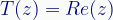
Where T(z) is defined as the function Re(z), which is a standard function that takes a complex number and returns the real part. (Its counterpart is Im(z), which returns the imaginary part. Note that both functions return real numbers.)

Figure 2. The space before and after the Real transform.

The result of the transformation is the one-dimensional real number line; the 2D complex plane collapses to a 1D line. All vectors “lie down” on the X-axis.

This, as mentioned, leaves the 2D space unmapped, and many vectors from that space end up mapped to the same vector.

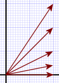
Figure 2a.

Notice that the vectors already aligned with the X-axis don’t move. This fact, that some vectors don’t move under some transformation, becomes hugely important later under the heading of eigenvectors.

In Figure 2a (which is before transform), all five vectors shown, after transformation, end up as the bottom vector that’s already lying directly on the X-axis. They all map to the same result vector.

That bottom vector doesn’t change and ends up as itself. Therefore, that bottom vector is an eigenvector of the Real transformation because it doesn’t change under that transformation. (There’s a bit more to it than that, but that’ll do for now. I have post coming later about eigenvectors and eigenvalues.)

§

We can also imagine a transformation (call it Zero) that collapses all vectors to the zero vector:

This (rather useless operation) reduces the entire space to a zero-D space — a single point.

Figure 3. The space before and after the Zero transform.

(Normally, transformations are not quite so reductive. These trivial examples serve to illustrate the notation and introduce the basic idea of a transform.)

§ §

In linear algebra, there are two important rules with regard to the allowed types of transformation:

• Firstly, the origin must remain in place; it never transforms. The zero vector remains the zero vector under transformation.

• Secondly, the transform must be linear, meaning it must preserve straight lines. Note that grid lines do not have to remain orthogonal (at right angles) or in any particular orientation — just straight.

§ §

The Null, Real, and Zero, transformation all obey these rules. The Real transformation collapses the vertical axis, and the Zero transform collapses both, but, they remain straight in the limit.

Speaking of which, if we think of the Zero transform as taking place over time, we see the vectors all shrink proportionally until they’re all zero. During this, the origin remains centered, and the axes remain straight. This implies another kind of transformation, Scale, that shrinks or expands all vectors proportionally by a factor:

The transform takes a scaling factor, sf, that determines how much to shrink (sf < 1.0) or expand (sf > 1.0) the vectors.

Figure 4. The space before and after a Scale(0.5) transform.

Note that, in reality, the “after” image should be covered with a half-sized grid, but in these examples I only transform the visible part of the “before” space to help illustrate the transform. Just remember that the transform includes the entire space.

§

Another legitimate transformation is a rotation, call it Rotate, that takes an angle, θ (theta), that specifies how much to rotate the space.

Rotate is always around the origin, which preserves the origin, and rotation also preserves straight lines.

Figure 5. The space before and after a Rotate(30) transform.

(Again, I’m only transforming the visible part of the “before” space. In reality the entire space is transformed.)

A rotation transform can include a scale transform, so:

Transform T takes a complex number, z, an angle, θ, and a scaling factor, sf. The definition assumes another transform, R, that takes the number and the angle and does the rotation transform. The resulting vector is then scaled by sf.

Figure 6. The space before and after a RotateScale(30, 0.5) transform.

As we’ll explore in the next post, there are various ways to accomplish these transforms, but all of them can be represented by square matrices (which is how I’ve done all the images you see here). To give you a taste of what such a matrix looks like, here’s the matrix for the RotateScale transform:

I won’t, in this series, explain exactly how this works because I’ve already covered that ground. See the Matrix Rotation and Matrix Magic posts.

§

We’ve seen transforms collapse axes, scale, or rotate (or do nothing). There are two additional transforms that preserve the straightness of axes.

First, note that above we had one transform that scaled the whole space, and another that collapsed one axis. The collapse is actually a scaling of that axis to zero. We can also scale one axis to some scaling factor:

Figure 7a. The space before and after a ScaleY(0.25) transform.

We can shrink or expand along any axis. The above scales the Y-axis, the below the X-axis:

Figure 7b. The space before and after a ScaleX(0.25) transform.

We can also scale on a diagonal:

Figure 8. The space before and after a Lorentz(0.5) transform.

In fact, this is the same transformation we see under a Lorentz transformation — the transformation we see of a frame moving relative to us. The example above represents the frame shift due to moving at 0.5 c.

§

The last transformation I’ll show you is a shear:

Figure 9. The space before and after a Shear(M) transform.

Note that, unlike the Lorentz transform, which rotates both axes, a shear only rotates one axis (in this case the Y-axis). The other axis just “slides” (or shears, hence the name).

It may not mean much right now, but the last two transforms (as far as I know) are pretty strictly matrix transforms. That’s why Shear(M) takes a matrix — it’s the only way to easily specify the transform.

To repeat an important point, a linear transformation preserves the straightness of the axes, but (as in the last two cases) need not preserve angles. The prior transforms all maintained the 90° orientation of the axes, but the last two obviously don’t.

§ §

The main point is that a transformation implicitly applies to all vectors in the space. The red grid in the examples stands in for all the vectors in the space.

In fact, we can use transforms to smoothly transform a continuous space:

Figure Bender (no one can). Before and after a shear transform.

Note that I arranged to have the pixels that were shifted off to the left be wrapped around to the right so we can see them — that is not part of the transform. To show it properly would require enlarging the after space to the left.

§ §

That’s enough for this time. Next time we’ll get into these transforms as operators on the space and talk about how they’re implemented.

I highly recommend, in general, Grant Sanderson’s ThreeBlueOneBrown YouTube channel for learning about mathematics in a fun visual way. It’s one of the best math channels around.

In particular I recommend his Linear Algebra playlist which introduces linear algebra in fairly short videos with outstanding animations and explanations. I’m deeply indebted to the channel and this series for helping me understand this stuff at a much deeper, more fundamental, level.

There are many other free resources available. Even Wikipedia has a lot, although it’s not always the best resource for beginners. It is pretty great once one gets rolling, though.

Stay transformed, my friends! Go forth and spread beauty and light.

∇