 This is the first of a series of posts exploring the mysterious Schrödinger Equation — a central player of quantum mechanics. Previous QM-101 posts have covered important foundational topics. Now it’s time to begin exploring that infamous, and perhaps intimidating, equation.
We’ll start with something similar, a classical equation that, among other things, governs how heat diffuses through a material. For simplicity, we’ll first consider a one-dimensional example — a thin metal rod. (Not truly one-dimensional, but reasonably close.)
Traveller’s Advisory: Math and graphs ahead!
For reference in what follows, here is a common version of the (time dependent) Schrödinger Equation:
![\displaystyle{i}\hbar\frac{\partial}{\partial{t}}\;\Psi(x,\!t)=-\left[\frac{\hbar^2}{2m}\,\frac{\partial^2}{\partial{x}^2}+V(x,\!t)\right]\Psi(x,\!t)](https://s0.wp.com/latex.php?latex=%5Cdisplaystyle%7Bi%7D%5Chbar%5Cfrac%7B%5Cpartial%7D%7B%5Cpartial%7Bt%7D%7D%5C%3B%5CPsi%28x%2C%5C%21t%29%3D-%5Cleft%5B%5Cfrac%7B%5Chbar%5E2%7D%7B2m%7D%5C%2C%5Cfrac%7B%5Cpartial%5E2%7D%7B%5Cpartial%7Bx%7D%5E2%7D%2BV%28x%2C%5C%21t%29%5Cright%5D%5CPsi%28x%2C%5C%21t%29+&bg=f9fbf9&fg=000099&s=0&c=20201002)
This post isn’t about that equation but this one:

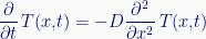
It’s a general classical diffusion equation that applies to many physical systems. For instance, how heat diffuses through a body. Note the general similarity between the two equations. On the left of the equals sign, both contain a (partial, ∂) derivative over time. On the right, both contain a second derivative (also partial, ∂²) over space.
On the far left of the Schrödinger Equation, the imaginary unit, i, and Planck’s constant, ħ (h-bar), distinguish it as a quantum equation. So does the wavefunction, Psi (Ψ). The equivalent in the diffusion equation is the temperature function, T. Note that both functions take two parameters, x and t. Both the wavefunction and the temperature function depend on space and time.
What matters here is how both equations govern the behavior of their functions by equating their first derivative over time with their second derivative over space. The classical example of heat diffusion offers an intuition into how the Schrödinger Equation treats the more mysterious quantum wavefunction.
We start with what it means to take the first or second derivative of a function over time or space. Given some function with a smooth curve (on a graph), the derivative of that function is a different curve representing the first one’s slope at each point.

Figure 1. Graph of the function f(x)=x³ [red line] and its first, second, and third, derivatives [green, blue, and purple lines, respectively].
Figure 1 shows the curve of a simple function, x³ (red), along with its 1st, 2nd, and 3rd, derivatives (green, blue, and purple, respectively). Each is the (first) derivative of the one before.
The red curve, viewed left to right, always moves upwards. Therefore, its slope is always positive, and its derivative (green) always has a positive value. Except at x=0, where the red curve is momentarily flat. The green curve is momentarily zero at this point. One value of derivatives is that zero values in the derivative indicate where the base curve is flat. These often indicate a peak (maximum) or valley (minimum).
The slope of the green curve left of center is downwards — negative. To the right of center, it’s upwards — positive. Therefore, its derivative (blue) is negative on the left and positive on the right. Note things become linear at this point (having gone from x³ to x² to x¹, which is just x). The blue line crosses the X-axis at zero, right where the green line touches it. This zero in the derivative again indicates a flat point in the base curve, and here it does indicate a minimum (a valley) in the green curve.
Because it’s straight, the slope of the blue line is constant, so its derivative (purple curve) is a constant value (in this case six). Any curve similar to the one we started with eventually derives to a constant slope and finally to a constant. The derivative of a constant is zero (because the slope of a flat line is zero). Further derivatives are also zero (the derivative of zero is zero).
Some functions, however, are endlessly derivable. They never approach a constant value (let alone zero). For instance, the function we’ll use as our temperature function.
§
More precisely, the simple equation that, along with parameters, describes the distribution of temperature in a “one dimensional” rod. Our simple model is governed by a Gaussian distribution — more familiarly known as a bell curve:
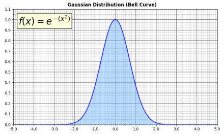
Figure 2. Basic Gaussian function (exponential).
Note that it’s the area under the curve (the blue region) that’s usually of interest with Gaussian distributions. In our case, it will represent the amount of heat present along a thin iron rod.
The basic equation is simply:
Yet another application for the exponential function! [See these posts.] We can parameterize the basic equation to control the Gaussian function’s height, width, and center point:

Where A sets the amplitude (height), B sets the center point, and C sets the width. Below are five instances of a Gaussian curve, each with a different height, width, and center point. They progress from tall and narrow (red) to short and wide (black):

Figure 3. Gaussian function with different A,B,C parameters.
Note that the width parameter, C, controls where the curve goes below 0.6 of its height. Note also these parameters are generally independent. A tall curve can be wide or narrow. So can a short one.
Seen as a temperature function, the height (the y value) represents how hot the rod is at that point (at that x value). Our starting state assumes the heat is concentrated in a small area in the center of the rod. (We assume it was rapidly heated with a blow torch or laser.) In such a case, the heat spreads out (diffuses) over time until the rod reaches equilibrium — the same temperature throughout.
The heat diffusion equation defines the spread of heat over time. Initially the curve is skinny and tall, indicating the heat concentrated in the center. Over time the height drops (rapidly), and the curve spreads out as the heat diffuses through the rod. Eventually the curve is flat — the rod at equilibrium.
[There are complications. The rod eventually settles at room temperature, whatever that is. If the heat of the experiment, once fully spread through the rod, is greater than room temperature, the rod radiates it away. Of course, the rod can never cool lower than room temperature. (In all cases here, assuming no other influence on the rod.)]
§ §
Understanding how this works requires understanding the derivatives in the diffusion equation. We need the first derivative over time and the second derivative over space. The latter is a bit easier to understand, so we’ll start there.
A derivative is the slope of a curve, so think about a hill. Our data is the ground height of as many points as possible. (Ideally, all the points.) This gives us a hill function that, for any x, returns the ground height at that point:
The first derivative of the hill function is a different function that, for any x, gives us the slope at that point (not the height). Slope is the rate of change in the height as we move around the hill:

It tells us how steep the slope is.
The second derivative of the hill function is yet another function that, for any x, returns the curvature of the hill at that point — the rate of change in the slope as we move along:

It tells us whether the slope is getting steeper or leveling out.

Figure 4. Curves for distance, velocity, and acceleration.
Figure 4 is intended for the next section, but it can also represent our hill as seen from the side. The red curve (labeled “distance”) is the hill’s height, the blue curve (“velocity”) is the 1st derivative (the hill’s slope), and the green curve (“acceleration”) is the 2nd derivative (the hill’s curvature).
Note how the slope (blue) peaks where the hill is steepest. But the curvature (green) is highest at the beginning and end of the slope — positive at the base, negative near the top.
We can tell the hill is momentarily straight in the middle of the incline because the curvature is positive in the beginning and negative approaching the top. It’s zero where it crosses the X-axis. That zero-crossing also indicates the max of the blue steepness curve. The hill is steepest at that point.
§
Actually, Figure 4 is a graph of motion, for instance of a car. The height of the red curve represents (as labeled) the distance traveled. The horizontal axis is time. Note this differs from the hill analogy where the horizontal axis was horizonal distance. This motion diagram is similar to spacetime diagrams, but instead of time running upwards, it runs left-to-right.
The distance grows slowly at first, increases quickly during the middle of the trip, and slows down at the end. The “car function” returns a distance traveled given some time t:

The first derivative returns the rate of change in distance — we call it speed or velocity. Mathematically, distance over time. For example, meters per second or miles per hour:

It tells us how fast or slow we’re going.
The second derivative returns the rate of change in velocity — we call it acceleration. Mathematically, distance over time-squared, or velocity over time.

Are we speeding up or slowing down?
§
Derivatives, as their name implies, are derived qualities. Hills seem to have physical steepness, but the reality is just ground height. Steepness derives from that. Curvature is doubly derived. Yet both represent physical truths. Climbing a steep hill is hard.
Velocity and acceleration in motion are similarly derived (yet represent clear physical truths). External forces play an important role in motion, of course, but they aren’t needed in this simplified case.
§ §
In summary, given some equation, there is a chain of derivatives that either ultimately derives to a constant (and then zero) or that continues indefinitely, sometimes cyclically (as with sin derivatives). As the hill and car examples show, for some equations, derivatives add slopes while for others, as in Figure 1, derivatives remove slopes.
The derivative chain behind Figure 1 is:

Note the alternate way of writing this:

Both say the same thing. The latter is a bit more flexible.
§ §
A time derivative involves rate of change over time. Going back to the hill, imagine the hill changing over time — wearing down and broadening. The time derivative tells us whether this evolution is fast (steep) or slow (shallow). This means the hill function takes a time parameter, t, in addition to the location parameter, x.
If the time derivative is zero, the hill isn’t changing.
As you’ll see, while our temperature function has an obvious x, it lacks a t parameter. The A (height) and C (width) parameters are what change over time, and our equation doesn’t address that. This is long enough that I’ll ignore it for now. It doesn’t affect the key point.
§ §
Here’s our temperature equation:
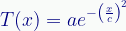
We’ll assume the curve is centered, so we don’t care about the B parameter (it will always be zero). We do need the a and c parameters (which have been demoted to lowercase). As just mentioned, they change over time, but at any given instant they’re constants.
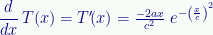
We have some interest in the first derivative over space (over x):
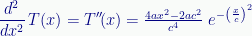
Mostly to get the second spatial derivative, the one required by the heat diffusion equation:
The third derivative is also of some interest:

You might notice that the original exponential function keeps appearing on the right of the derivatives. That’s a prominent characteristic of the exponential function. Its derivative always contains itself.
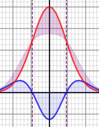
Here’s a graph of the heat equation (red) and its three derivatives:

Figure 5. Gaussian (a=3.0, c=1.0) with 1st, 2nd, and 3rd, derivatives.
The dashed lines mark where the second (purple) and third (green) derivatives cross the X-axis — where these functions are zero. We use these zero points (called roots) to locate minima and maxima.
The roots for the second derivative (purple dashed lines) indicate the max and min points on the first derivative (blue) and therefore the points of max and min slope on the main curve (red). They also mark inflection points where that curve switches from positive to negative curvature (and then back to positive at the second root). Quite a lot for a pair of zeros.
The roots of the third derivative (green dashed line) mark second derivative maxima. These are points of maximum curvature of the red curve. There is also a root at x=0, another point of maximum curvature. (The first derivative’s only root is x=0. The point where the red curve switches from positive to negative slope.)
The second derivative (purple) has a positive value on the sides and a negative value in the middle. Recall the diffusion equation has a second spatial derivative on its right-hand side:
Now consider the effect of combining the temperature curve with its second spatial derivative:

Figure 6. The point of this post! The purple shading on the red curve shows the effect on it of the 2nd derivative (blue curve).
The positive outside pulls the cool parts up while the negative middle pulls the hot part down. In particular, note the effect is especially strong in the high-curvature areas of the red line (such as the peak). Large values in the (blue) second derivative indicate high-curvature areas in the (red) base function.
The result is a shorter, broader curve. Over time, the heat spreads out. Eventually it equalizes.
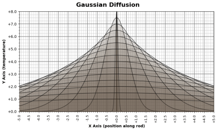
Figure 7. Over time, heat spreads out (equalizes) through the rod.
The “force” affecting the heat at any point depends on the second derivative — the curvature of the heat field at that point. It amounts to a measure of how much a given point varies, not just from its neighbors, but from the average of its neighbors.
The diffusion equation equates this, through the constant D, to the time derivative — how the value of that point is changing over time. The implication is that points that stand out from the average change rapidly towards the average.
[Keep in mind it’s curvature — not slope — that’s important. A rod heated at one end and cooled at the other equalizes to a flat slope from hot to cold. That’s a stable solution to the heat equation because the curvature of a flat slope is zero. Which makes the time derivative zero.]
§ §
The point: The Schrödinger Equation has a similar effect on quantum wavefunctions. This is why, for instance, when a particle is localized by an interaction, its wavefunction begins to spread out immediately afterwards.
Generally speaking, unless confined, quantum wavefunctions spread out over time. Position in space spreads, but other quantum properties can diffuse as well.
But not always. Quantum mechanics depends on complex numbers, so wavefunctions can also oscillate and interfere. But those are topics for the future. Next time I’ll explore this spreading out in more detail and add a dimension.
Stay Gaussy, my friends! Go forth and spread beauty and light.
∇


November 8th, 2022 at 7:50 am
Appendix 1
This appendix shows step-by-step how to calculate the derivatives of exponential functions.
We’ll start with the base equation:
We use a special instance of the chain rule to derive an exponential function. Recall that the basic chain rule is:
For exponential functions we have:
Because the derivative of the exponential function is the exponential function. That’s kind of its whole deal. It’s its own derivative. Few functions can say that.
So, for the temperature equation, we get the first derivative like this:
Which, rearranged a little is the first derivative shown above:
To derive this one, we’ll need the product rule since there are now two factors that are functions of x. The product rule is:
In the case of the first derivative, the two factors are:
So, we start with:
We factor out the exponential and do the derivative (x vanishes), which gives us:
Then we do the multiplication on the left of the plus and multiply the right side by c²/c² to make the denominators match:
And again, with a little rearranging, we have the second derivative shown above:
This one also has two factors that are functions of x, so deriving it is similar to the previous one. Here the two factors are:
The second one is the same, of course. The exponential function keeps reappearing in its derivatives! Given these functions, we derive them:
As before, we factor out the exponential and do the derivative (this time we still get a function of x):
Again, we do the multiplication on the left and multiply the right side of the plus sign by c²/c² to make the denominators match:
The second and third terms inside the parentheses match, so we can reduce this to the third derivative shown in the post:
We won’t derive it further (although we could; endlessly). We just wanted this to calculate its roots. Those tell us where the minima and maxima of the second derivative are, and those indicate the maximum curvature parts of the base function (which, admittedly, falls into the Nice to Know category).
§
The temperature equation isn’t parameterized for time (yet), so there’s no way to calculate the time derivative at this, um, time.
November 8th, 2022 at 7:50 am
Appendix 2
We want to calculate the roots of the derivatives — points where the value is zero. So we will.
Given the requirement that a and c are never zero, the base equation clearly never vanishes (becomes zero):
As x grows larger, x/c grows larger, and the function’s value approaches — but never reaches — zero. The squaring causes negative x values to act like positive ones, so the function is symmetrical.
Since the exponential never vanishes, for the derivatives to vanish requires their first parts, the polynomial, vanish. So, we just need to see if and where they do.
The first one is easy. Rewritten slightly, it’s obvious that for this to be true…
…the left part is a constant, so the only way for this function to vanish is for x itself to be zero. And indeed, the first derivative has just the one root, x=0.
§
The second derivative is only slightly less obvious:
We again factor out the constants, ignore them (they’ll never be zero), and focus on what remains:
So, the second derivative has two roots, x=±c/v2. We can see that x=0 is not a root because the function has a value at that point.
§
The third derivative is more of the same. Absent the exponential, we have:
We again ignore the factored-out constants focus on what remains:
So, the third derivative has the two roots ±v3/2×c as well as one at x=0, because we can see the function vanishes there. Note how the roots for these two derivatives depend on c (but not on a). They depend on the width of the base curve.
And that’s it. QED?
November 8th, 2022 at 7:59 am
How’s that for a change of pace? 😁
November 8th, 2022 at 10:02 am
I hope you did, too.
Gotta say, I love living in the boonies. Walked in, stood behind one person for less than a minute, checked in, got my ballot, marked it, put it in the machine, and got my sticker, all in just a few painless minutes. Small Cities Rule!
November 8th, 2022 at 3:11 pm
Yes! “Climbing a steep hill is hard.” Say more about that.
November 8th, 2022 at 5:09 pm
Heh, “is hard” kind of says it all!
I still remember my seventh-grade science teacher telling us how, in physics, “work” requires moving weight against gravity. Just pushing weight around on a level surface, technically, wasn’t “work”.
Science is weird! 😆
November 10th, 2022 at 7:48 am
[…] Last time I began exploring the similarity between the Schrödinger equation and a classical heat diffusion equation. In both cases, valid solutions push the high curvature parts of their respective functions towards flatness. The effect is generally an averaging out in whatever space the function occupies. […]
November 11th, 2022 at 12:27 pm
[…] last two posts were heavy on the math, so I promise (other than the date thing) no math in this […]
September 20th, 2023 at 2:28 pm
[…] been a while, but the two previous posts in this series (this one and this one) explored the mechanism behind partial differential equations that equate the time […]