November 10, 2022

QM 101: Diffusion in 2D

Last time I began exploring the similarity between the Schrödinger equation and a classical heat diffusion equation. In both cases, valid solutions push the high curvature parts of their respective functions towards flatness. The effect is generally an averaging out in whatever space the function occupies.

Both equations involve partial derivatives, and I ignored that in our simple one-dimensional case. Regular derivatives were sufficient. But math in two dimensions, let alone in three, requires partial derivatives.

Which were yet another hill I faced trying to understand physics math. If they are as opaque to you as they were to me, read on…

This post assumes you are at least basically familiar with regular derivatives — derived functions of other functions that represent the slope of the base function. Or the slope of the slope (slope²), or the slope of the slope of the slope (slope³). Et cetera. These sound progressively artificial, but they often represent real-world effects. For example, we feel distance-over-time² — a second derivative — by its common name, acceleration.

Second derivatives, which we can think of as indicating the curvature of a function, also matter in the Schrödinger Equation:

$\displaystyle{i}\hbar\frac{\partial}{\partial{t}}\;\Psi(x,\!t)=-\left[\frac{\hbar^2}{2m}\,\frac{\partial^2}{\partial{x}^2}+V(x,\!t)\right]\Psi(x,\!t)$

And in the heat diffusion equation:

$\displaystyle\frac{\partial}{\partial{t}}\,{T}(x,\!t)={D}\frac{\partial^{2}}{\partial{x}^{2}}\,{T}(x,\!t)$

In this case, it’s something-over-space² — a spatial (second) derivative. In the case of our heat example, the something is heat energy. In the case of the Schrödinger equation, it’s probability amplitude.

More importantly, both equations, to be useful, must be applied to our three-dimensional space. Which is where partial derivatives come into play. Let’s start with the notation. Regular derivatives over x look like this:

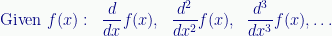
$\displaystyle\textrm{Given }f(x):\;\;\frac{d}{dx}f(x),\;\;\frac{d^2}{dx^2}f(x),\;\;\frac{d^3}{dx^3}f(x),\ldots$

While partial derivatives (again over x) look like this:

$\displaystyle\textrm{Given }f(x,\!y):\,\frac{\partial}{\partial{x}}f(x,\!y),\;\frac{\partial^2}{\partial{x^2}}f(x,\!y),\;\frac{\partial^3}{\partial{x^3}}f(x,\!y),\ldots$

Derivatives over different axes just use the appropriate variable. Notice how the function takes two parameters. That’s why partial derivatives. They’re (partial) derivatives over one of the variables in a multi-variable function.

For instance, in three-dimensional space, with X, Y, and Z:

$\displaystyle\textrm{Given }f(x,\!y,\!z):\;\frac{\partial}{\partial{x}}f(x,\!y,\!z),\;\;\frac{\partial^2}{\partial{x^2}}f(x,\!y,\!z)$

Which are the first and second derivatives over the X axis in 3D space. They provide, respectively, the “slope” and “curvature” of some real-world property, but only in the X direction.

Obviously, this is indeed partial information. To have value, we’d also need the partial derivatives along the Y and Z axes. (And sometimes along the time axis, as in the diffusion and Schrödinger equations.)

Three dimensional applications of partial derivatives are so common mathematicians and physicists abbreviate it with a special symbol:

$\displaystyle\nabla=\hat{x}\frac{\partial}{\partial{x}}+\hat{y}\frac{\partial}{\partial{y}}+\hat{z}\frac{\partial}{\partial{z}}$

Which combines the (first) partial derivatives along the three dimensions of space into a slope value that represents all three. Likewise, we have:

$\displaystyle\nabla^2=\hat{x}\frac{\partial^2}{\partial{x^2}}+\hat{y}\frac{\partial^2}{\partial{y^2}}+\hat{z}\frac{\partial^2}{\partial{z^2}}$

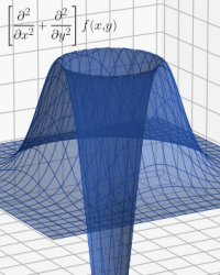
Which combines the second partial derivatives, giving us the three-dimensional curvature of the field.

This symbol, called nabla or del, is an operator, so using it requires applying it to some function:

$\displaystyle\nabla^2\,{T}(x,y,z)=\left[\hat{x}\frac{\partial^2}{\partial{x^2}}+\hat{y}\frac{\partial^2}{\partial{y^2}}+\hat{z}\frac{\partial^2}{\partial{z^2}}\right]T(x,y,z)$

Which applies each of the partial differentials to the three-dimensional function T and sums the results.

§ §

Recall how in the Schrödinger and heat diffusion equations the second spatial derivative, the curvature of the field, determines the “force” pulling it towards flatness. (In cases so far discussed. The complex number math in quantum mechanics makes it a bit more involved.)

The important generality is that second derivatives tell us whether the rate of change of some system is increasing or decreasing. Often, the rate of change is less important than whether that rate grows or shrinks. Especially rapidly. A speed of 100 miles per hour isn’t dangerous. Rapidly slowing to 3 miles per hour is fatal.

So, second derivatives, which think of as curvature, are important. It’s worth taking a moment to describe what’s really going on when it comes to curvature — what it tells us about a point in space.

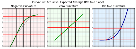
Figure 1. Three curves with positive slope and different curvatures.

Figure 1 shows three curves. They have no particular meaning, they’re just the curves of some random function. Or rather, part of those curves. Assume they continue beyond what’s shown; we’re focusing only on segments of interest.

All three curves have positive slope — they go upwards (have more positive Y values) from left to right. But each, per their captions, illustrates a different kind of curvature.

Zero curvature means the slope isn’t changing. Positive curvature means it’s growing more positive; negative means it’s growing less positive (and therefore more negative). Any slope, positive, negative, or flat, can have negative, zero, or positive curvature.

Figure 2. Three curves with negative slope and different curvatures.

Figure 2 shows a situation similar to Figure 1, but with negative slopes. And since slope isn’t important, the next section treats these two diagrams as if they were one. Only the curvature — the second derivative — matters.

Notice that each curve has three evenly spaced vertical gray lines. These intersect the curve at three red points along the curve. There are also three horizontal red lines that intersect the points.

The red lines are evenly spaced only in the center panel. In the left and right panels, the middle red line is off-center. Also, the red points in the center panel line up in a straight line. (The curve is straight, and the points are on the curve, so they have to line up.) But in the left and right panels, the middle point is either above or below a straight line between the outside points.

The straight line represents the average. If the middle point is on a straight line between its “nearest neighbors” then its value matches the average of those neighbors. (This is calculus, so the concept of “nearest neighbors” involves the limit as they get infinitely close.)

The bottom line is that when a point’s curvature is negative, it’s above the local average, and when its curvature is positive, it’s below the local average.

If we view the curves as translation or transfer functions, we can think of the three vertical gray lines as inputs and the three horizontal red lines as outputs. When the inputs are evenly spaced, if the outputs are also evenly spaced, the transfer function is linear. (The spacing doesn’t have to be the same, just even.)

But if the outputs are not evenly spaced, then the transfer function is nonlinear. Because the transfer function has curvature. Here again the second derivative tells us something. If it’s non-zero, the system it describes is nonlinear (at least in that area).

§ §

Because it’s easy to show graphically, I’ll discuss a 2D example of the heat function. The intent is to provide an intuition for the much harder to render three-dimensional case.

Here is what our 2D Gaussian heat function looks like:

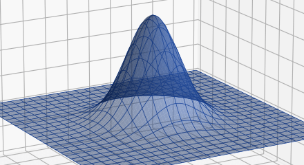
Figure 3. Two-dimensional Gaussian function.

Rather than a rod, a flat plate we treat two-dimensionally. (Assume the center of the plate is suddenly heated, for instance by a blowtorch or laser.) The height of the graph indicates the heat at that point on the plate.

A parameterized two-dimensional Gaussian looks like this:

$\displaystyle{g}(x,y)={ae}^{-\left(\frac{x^2+y^2}{c^2}\right)}$

It’s much like the one-dimensional Gaussian, just with an added y parameter. And since it has two parameters, x and y, there are two partial derivatives, one over x:

$\displaystyle{g}_x'(x,y)=\frac{\partial}{\partial{x}}{ae}^{-\left(\frac{x^2+y^2}{c^2}\right)}=\frac{-2ax}{c^2}\;{e}^{-\left(\frac{x^2+y^2}{c^2}\right)}$

And one over y:

$\displaystyle{g}_y'(x,y)=\frac{\partial}{\partial{y}}{ae}^{-\left(\frac{x^2+y^2}{c^2}\right)}=\frac{-2ay}{c^2}\;{e}^{-\left(\frac{x^2+y^2}{c^2}\right)}$

They’re very similar, just differing in whether they pull x or y out of the exponential. In the process, since the other variable (y or x) is viewed as a constant, its derivative is zero and it vanishes.

Likewise, there are two partial second derivatives, one over x:

$\displaystyle{g}_x''(x,y)=\frac{\partial^2}{\partial{x^2}}{ae}^{-\left(\frac{x^2+y^2}{c^2}\right)}=\frac{4ax^2-2ac^2}{c^4}\;{e}^{-\left(\frac{x^2+y^2}{c^2}\right)}$

And one over y:

$\displaystyle{g}_y''(x,y)=\frac{\partial^2}{\partial{y^2}}{ae}^{-\left(\frac{x^2+y^2}{c^2}\right)}=\frac{4ay^2-2ac^2}{c^4}\;{e}^{-\left(\frac{x^2+y^2}{c^2}\right)}$

Again, only differing in whether they pull x or y out of the exponential.

§ §

So, a partial derivative is just taking a regular derivative over one of the variables in a multi-variable function while treating the other variables as constants.

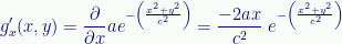
Figure 4 is a graph of the first partial derivative over x (note that height now indicates the slope of the 2D Gaussian “hill”):

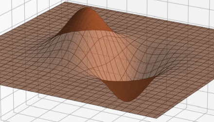
Figure 4. The 2D Gaussian first partial derivative over x.

The derivative is taken in the positive direction along the X axis (which runs from the upper left to the lower right), so the positive bump on the left represents the “uphill” (positive) slope of the Gaussian while the negative dip on the right side indicates the “downhill” (negative) slope. The two are symmetrical because the sides of the Gaussian are symmetrical.

Given the 2D Gaussian function, g(x,y), the calculation for Figure 4 is:

$\displaystyle\frac{\partial\,{g}(x,y)}{\partial{x}}=\frac{-2ax}{c^2}\;{e}^{-\left(\frac{x^2+y^2}{c^2}\right)}$

Figure 4 is a two-dimensional version of the first derivative shown in Figure 5 of the previous post. This is readily apparent if we view it head on from the front:

Figure 4a. The 2D Gaussian first partial derivative over x seen along the Y axis with the X axis running from left (-x) to right (+x).

Two points of interest: Firstly, the derivative is zero at x=0 (all along the Y axis). That’s because, if we approach the hill strictly along the Y axis, the steepness in the X direction orthogonal to us. Secondly, the bump and dip taper off in the Y direction.

We see this clearly by viewing from the side:

Figure 4b. The 2D Gaussian first partial derivative over x seen along the X axis with the Y axis running from left (-y) to right (+y).

If we approach the hill parallel to, but some small distance way from, the X axis, we climb only part of the hill. Which isn’t as steep as climbing the whole thing, and the tapering of the lobes reflects that.

The first partial derivative over y is the same except rotated 90 degrees:

Figure 5. The 2D Gaussian first partial derivative over y.

In this case, we’re moving along the Y axis, so we first go uphill and then downhill. (Sharp-eyed readers will spot I’ve reversed the direction along the Y axis. That way the bump doesn’t block our view of the dip.) Everything here is exactly the same as above, just rotated 90 degrees.

Recall that our interest in the first spatial derivative was mainly to derive it to get the second spatial derivative needed by the diffusion equation (and the Schrödinger equation).

Here’s a graph of the 2D Gaussian second partial derivative over x (now height indicates the curvature of the slope of the Gaussian hill):

Figure 6. The 2D Gaussian second partial derivative over x.

Again, it’s a two-dimensional version of the second derivative we saw in the previous post.

Given, again, the 2D Gaussian function, g(x,y), the calculation for Figure 6 is:

$\displaystyle\frac{\partial^2\,{g}(x,y)}{\partial{x^2}}=\frac{4ax^2-2ac^2}{c^4}\;{e}^{-\left(\frac{x^2+y^2}{c^2}\right)}$

As with the first derivative, the similarity to the one-dimensional case is readily apparent when viewed directly from the front:

Figure 6a. The 2D Gaussian second partial derivative over x seen along the Y axis with the X axis running from left (-x) to right (+x).

It’s not obvious in the perspective view, but Figure 6a shows the symmetry. Both positive bumps are the same height. The valley in the middle reflects the negative curvature of the crest of the Gaussian (the top of the hill). The narrower the Gaussian, the deeper (more negative) this valley gets.

The symmetry from the side is similar to the first derivative. Both have positive and negative lobes (bumps and dips):

Figure 6b. The 2D Gaussian second partial derivative over x seen along the X axis with the Y axis running from left (-y) to right (+y).

You can see how it tapers off along the Y axis. Note also the Gaussian shape.

The second partial derivative over y is similar but rotated 90 degrees.

§ §

The point of all this (other than pretty 3D graphs) is that something interesting happens when we add the second derivatives — something that doesn’t happen with the first derivatives.

Here’s what it looks like when we sum the x and y partial derivatives:

Figure 7. The sum of 2D Gaussian first partial derivatives.

This looks very much like Figure 4 or Figure 5, only rotated 45 degrees. The sum still retains a sense of directionality. It tells us the steepness of the hill but only in reference to a specific direction. Not much more helpful than the partial derivatives themselves.

But if we sum the second partial derivatives, we get:

Figure 8. The sum of 2D Gaussian second partial derivatives.

This has the same 360° symmetry as the original 2D Gaussian! More second derivative magic. It tells us that, regardless of how we approach the hill, it has positive curvature at the base and negative curvature at the crest.

The calculation for Figure 8 is:

$\displaystyle\left[\frac{\partial^2}{\partial{x^2}}+\frac{\partial^2}{\partial{y^2}}\right]{g}(x,y)=\frac{4ax^2+4ay^2-4ac^2}{c^4}\;{e}^{-\left(\frac{x^2+y^2}{c^2}\right)}$

And the effect this (now full) second derivative has on the original Gaussian is the same as discussed last time. That deep negative hole pulls the crest of the Gaussian hill down while that positive circular “crater ridge.” acts to pull the base of the hill up.

§ §

We end in much the same place as last time but having added a dimension. Hopefully, this helps you imagine this in three dimensions. (It’s a challenge to illustrate a 3D function let alone its derivatives.)

Now we can write a two-dimensional heat diffusion equation:

$\displaystyle\frac{\partial}{\partial{t}}\,{T}(x,y,\!t)={D}\left[\frac{\partial^{2}}{\partial{x}^{2}}+\frac{\partial^{2}}{\partial{y}^{2}}\right]{T}(x,y,\!t)$

And simplify it with the nabla operator:

$\displaystyle\frac{\partial}{\partial{t}}\,{T}(x,y,\!t)={D}\nabla^{2}\;{T}(x,y,\!t)$

(With the understanding it’s a two-dimensional application.)

Regardless of how we write it, the equation says the spatial curvature is proportional (through the constant D) to the rate of change over time. High curvature, rapid change. For diffusion equations and for the Schrödinger equation.

That’s the bottom line.

§ §

In future posts I’ll do the traditional thing and explain each part of the Schrödinger equation. I’ll explore what each part does in the context of this and the previous post.

I’ll also talk about the difference between the Schrödinger equation and the quantum wavefunction. I’ll dig into what a quantum wavefunction actually is (at least mathematically; no one knows what it is physically).

Stay partial, my friends! Go forth and spread beauty and light.

∇²∂

About Wyrd Smythe

The canonical fool on the hill watching the sunset and the rotation of the planet and thinking what he imagines are large thoughts. View all posts by Wyrd Smythe

This entry was posted on Thursday, November 10th, 2022 at 7:47 am and tagged with derivatives, exponential function, partial derivatives, QM101, Schrödinger Equation and posted in Math, Physics. You can follow any responses to this entry through the RSS 2.0 feed.

10 responses to “QM 101: Diffusion in 2D”

Wyrd Smythe
November 10th, 2022 at 8:01 am

Appendix 1

This appendix shows step-by-step how to calculate the derivatives used in the post.

Here’s the base equation:

$\displaystyle{g}(x,y)={ae}^{-\left(\frac{x^2+y^2}{c^2}\right)}$

Where a controls the amplitude and c controls the width. Since we’ll need it later, let’s start by deriving just the exponential. First, along the X axis:

$\displaystyle\frac{\partial}{\partial{x}}{e}^{-\left(\frac{x^2+y^2}{c^2}\right)}=\frac{-2x}{c^2}{e}^{-\left(\frac{x^2+y^2}{c^2}\right)}$

Then along the Y axis:

$\displaystyle\frac{\partial}{\partial{y}}{e}^{-\left(\frac{x^2+y^2}{c^2}\right)}=\frac{-2y}{c^2}{e}^{-\left(\frac{x^2+y^2}{c^2}\right)}$

The derivative uses the chain rule where we equate u to the exponent in the exponential:

$\displaystyle{u}=-\left(\frac{x^2+y^2}{c^2}\right)$

So, with u a function of x, we apply the chain rule:

$\displaystyle\frac{d}{dx}{e}^{u}=\frac{d}{dx}{e}^{u}\frac{d}{dx}{u}={e}^{u}\frac{d}{dx}{u}$

Because the derivative of an exponential is that exponential. Now we only need to derive:

$\displaystyle\frac{d}{dx}{u}=\frac{d}{dx}(-1)\frac{x^2+y^2}{c^2}=\frac{-2x}{c^2}$

With a similar derivation for y. Plugging these into the above, for x:

$\displaystyle\frac{d}{dx}{e}^{-\left(\frac{x^2+y^2}{c^2}\right)}={e}^{u}{u'}={e}^{-\left(\frac{x^2+y^2}{c^2}\right)}\left[\frac{-2x}{c^2}\right]$

Which, rearranged, is what’s shown above. The y derivation works the same way.

Deriving the base equation gives almost the same result, we just include the constant, a:

$\displaystyle\frac{\partial}{\partial{x}}{ae}^{-\left(\frac{x^2+y^2}{c^2}\right)}=\frac{-2ax}{c^2}{e}^{-\left(\frac{x^2+y^2}{c^2}\right)}$

With a similar one for y.

§

For the second derivative we need the product rule:

$\displaystyle{x}=\frac{d}{dx}u(x)v(x)=u(x)v'(x)+u'(x)v(x)$

Which is why we derived just the exponential for later. This is later. In the context of the product rule, we need to derive:

$\displaystyle{u}(x)=\frac{-2ax}{c^2},\;\;{v}(x)={e}^{-\left(\frac{x^2+y^2}{c^2}\right)}$

And we already know what v‘(x) is, so we just need u‘(x):

$\displaystyle\frac{d}{dx}u(x)=\frac{d}{dx}\left[\frac{-2ax}{c^2}\right]=\frac{-2a}{c^2}$

Putting it all together, for x:

$\displaystyle\frac{\partial}{\partial{x}}\left[\frac{-2ax}{c^2}{e}^{-\left(\frac{x^2+y^2}{c^2}\right)}\right]=\left[\frac{-2ax}{c^2}\frac{-2x}{c^2}{e}^{-\left(\frac{x^2+y^2}{c^2}\right)}\right]+\left[\frac{-2a}{c^2}{e}^{-\left(\frac{x^2+y^2}{c^2}\right)}\right]$

Extracting the common exponential, doing the multiplication on the left, and multiplying the right term by c²/c² to create a common denominator:

$\displaystyle\frac{\partial}{\partial{x}}\left[\frac{-2ax}{c^2}{e}^{-\left(\frac{x^2+y^2}{c^2}\right)}\right]=\left[\frac{4ax^2}{c^4}+\frac{-2ac^2}{c^4}\right]{e}^{-\left(\frac{x^2+y^2}{c^2}\right)}$

Cleaning it up we have the second derivation:

$\displaystyle\frac{\partial}{\partial{x}}\left[\frac{-2ax}{c^2}{e}^{-\left(\frac{x^2+y^2}{c^2}\right)}\right]=\frac{4ax^2-2ac^2}{c^4}{e}^{-\left(\frac{x^2+y^2}{c^2}\right)}$

With a similar one for y.

Reply
- Wyrd Smythe
  November 18th, 2022 at 12:53 am
  
  The third partial derivative over x is:
  
  $\displaystyle\frac{\partial^3}{\partial{x}^3}\left[{ae}^{-\left(\frac{x^2+y^2}{c^2}\right)}\right]=\frac{-8ax^3+12ac^2x}{c^6}\;{e}^{-\left(\frac{x^2+y^2}{c^2}\right)}$
  
  Deriving it is left as an exercise (but see Appendix1 in previous post).
  
  Reply
Wyrd Smythe
November 10th, 2022 at 8:02 am

Appendix 2

It’s worth digging into the mechanics of taking the derivative of the exponential function. It begins with the basic fact that the derivative of the exponential function is the exponential function:

$\displaystyle\frac{d}{dx}\,{e}^{x}={e}^{x}$

The slope of e^x at x is always just e^x. Note this is true when the exponent is just x. (We’ll sort of see why below.) If the exponent is an expression containing x, then the expression is a function of x, and the chain rule applies.

The chain rule is:

$\displaystyle\frac{d}{dx}\,f(g(x))={f'}(g(x))\cdot{g'}(x)$

If a function, f, depends on a sub-function, g, multiply the derivative of the outer function times the derivative of the inner function.

To see how this works, we can see what happens when we apply the chain rule to the basic exponential function (which we know derives to itself). We’ll treat the plain x in the exponent as a function, g(x), that just returns x:

Applying the chain rule and setting u=g(x) to simplify the exponential:

$\displaystyle\frac{d}{dx}\,{e}^{g(x)}=\frac{d}{du}\,{e}^{u}\,\cdot\,\frac{d}{dx}\,g(x)={e}^{u}\,\cdot\,\frac{d}{dx}\,{x}$

Since the derivative of x is just 1, we end up with, as expected, the original exponential. Rearranged a bit, this is a basic formula for deriving the exponential function:

$\displaystyle\frac{d}{dx}\,{e}^{u}=u'\;{e}^{u}$

Where u is some expression containing (at least one occurrence of) x. Just take the derivative of that expression and multiply it to the exponential.

With that understanding, let’s try this:

$\displaystyle\frac{d}{dx}\,{e}^{2x}=\frac{d}{dx}\,\left[{2x}\right]{e}^{2x}={2}\cdot{e}^{2x}$

Because the derivative of 2x is just 2.

Here’s one with a square of x, such as appears in the Gaussian exponential function:

$\displaystyle\frac{d}{dx}\,{e}^{x^2}=\frac{d}{dx}\,\left[{x}^{2}\right]{e}^{x^2}={2x}\cdot{e}^{x^2}$

Because the derivative of x² is 2x.

If there was a constant in front of the exponential, it just gets multiplied by the derived exponent:

$\displaystyle\frac{d}{dx}\,{ae}^{x^2}=\frac{d}{dx}\,\left[{x}^{2}\right]{ae}^{x^2}={2ax}\cdot{e}^{x^2}$

We can break this down as an instance of the product rule, which is:

$\displaystyle\frac{d}{dx}\,f(x)\,g(x)=f(x)g'(x)+f'(x)g(x)$

But since a is a constant, it derives to zero, so:

$\displaystyle\frac{d}{dx}{ae}^{x^2}\!=\!\left[{a}\cdot\frac{d}{dx}{e}^{x^2}\right]\!\!+\!\!\left[\frac{d}{dx}{a}\cdot{e}^{x^2}\right]\!=\!\left[2ax\cdot{e}^{x^2}\right]\!\!+\!\!\left[0\cdot{e}^{x^2}\right]$

Which gives us the result shown above.

Finally, note that, since a constant derives to zero, an exponential function with a constant exponent also derives to zero:

$\displaystyle\frac{d}{dx}\,{e}^{k}=\frac{d}{dx}\,\left[{k}\right]{e}^{k}={0e}^{k}=0$

Hopefully this helps make it clear how to derive more involved exponential functions!

Reply
Wyrd Smythe
November 10th, 2022 at 8:07 am

Looking at how this renders in the #%$&* WP Reader just breaks my heart. Most images are enlarged so they look crappy, but a few are left alone. Why? Don’t know. Because the #%$&* WP Reader is a piece of worthless crap? Yeah, probably that.

Reply
Mark Edward Jabbour
November 10th, 2022 at 8:50 am

They all look fine on my tablet, via the email. Which is different than the reader. And I can enlarge all and anything.

Each device (phone, tablet, laptop) I have presents the content differently.

It’s frustrating, yes. As well as the constant “upgrades “.

A constant race to be “better “ leads to wtf ! Why the hell did they do that?

Analytics?

Reply
- Wyrd Smythe
  November 10th, 2022 at 1:13 pm
  
  I… really, really, really hate WP software. It seems to be designed, built, and maintained, by idiots. (Back in the last century, software was perceived as the booming industry and a lot of people got into it who had no instinct or talent for it, which is why so much of it is so bad.) I just spent 20 minutes writing a reply and lost it because I accidentally hit a wrong key and this incompetent WP software can’t trap the exit and ask if I’m sure I want to just throw away 20 minutes work. Taking care with a user’s work is software development 101, and these fucks failed.)
  
  Speaking of which, were you looking at my post on my blog’s website (logosconcarne URL) or with the WordPress Reader (wordpress URL)? It’s only the latter that’s the problem.
  
  The comment I lost, I was off on a long-standing rant about the war between the original vision Tim Berners-Lee had for the web versus what it became. Not the fraud or commercialization or porn or social media, but just in how content is rendered. The original idea was that end users had a lot of control over how pages look. Artists and content developers wanted their stuff to look exactly as designed. Over time, they won, and the web became very complicated to allow artistic control in a medium that wasn’t originally designed for it.
  
  This is like a bad version of that. The WP Reader wants all posts to look identical, so it throws away a lot of the meta-information writers include (sometimes even bolding and italics get lost). For instance, my section marks (§) are supposed to be centered, but the WP Reader has them against the left margin. And now it’s enlarging most (but weirdly not all) images so they stretch from left margin to right margin (in the Reader). That blows them up and they look bad.
  
  [sigh] WordPress… just one more thorn in my side. I just finished a long round of emails with their support staff over an issue I had with the editor. Used to be interacting with WP Help always had a good result. That hasn’t been true in years now. It always ends in frustration and no fix.
  
  Reply
Mark Edward Jabbour
November 11th, 2022 at 10:33 am

hmmm … the “web” is not my preferred way to communicate, for sure. One thing for certain is – it’s unreliable. But now, it’s the way we (humans) communicate most. If it’s not the machine, it’s the person at the keyboard. Furthermore, now, it can be an algorithm. [Or a satellite. A bird? Space junk?]

Anyone of those three actors can go awry at any time for any number of reasons. Without intention.
For an Engineer, it must be super frustrating.

My psych-girl suggested to me once that I “lower my expectations”. That’s hard for me.

Hang in there. Have a good weekend. cheers.

Reply
- Wyrd Smythe
  November 11th, 2022 at 12:43 pm
  
  It’s said that communication is 55% visual (expression, posture, etc), 38% vocal (tone, inflection, etc), and only 7% verbal (or textual). So, most forms of online communication (like comments) are severely stunted in bandwidth. Writing is so much different from speaking! We all have a lifetime’s practice speaking, but not everyone has training and practice writing.
  
  Engineering, despite its reputation, is easy and relaxing compared to people. Not easy. Not relaxing. Most of them, anyway. The thing about math is that opinions don’t matter. Math is right or not. Generally the case with science or engineering, too. Electricity doesn’t care what you think.
  
  I’d guess psych-people, vested in helping people cope, focus on what is, and right enough, but I am ever nagged (and perhaps you are, too) about ought. My Weltschmerz sometimes reaches profound levels.
  
  Reply
Friday Notes (Nov 11, 2022) | Logos con carne
November 11th, 2022 at 12:27 pm

[…] last two posts were heavy on the math, so I promise (other than the date thing) no math in this one. But […]

Reply
Wyrd Smythe
November 17th, 2022 at 11:51 am

How’s this for synchronicity: One of the YouTube channels I follow just posted this video about partial derivatives:

Reply