 Last time I began explaining my “CD collection” analogy for entropy; here I’ll pick up where I left off (and hopefully finish — I seem to be writing a lot of trilogies these days). There’s more to say about macro-states, and I want also to get into the idea of indexing.
I make no claims for creativity with this analogy. It’s just a concrete instance of the mathematical abstraction of a totally sorted list (with no duplicates). A box of numbered index cards would work just as well. There are myriad parallel examples.
One goal here is to link the abstraction with reality.
To summarize and review:
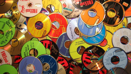
◊ There is a CD collection of at least 5,000 CDs (no duplicates). The collection has a sort order defined on it. The nature of the ordering doesn’t matter, only that some property of the CDs allows unambiguous ordering.
◊ We define the sort degree as the minimum number of moves required to restore the collection to sorted order. When fully sorted, the sort degree is zero. The sort degree is our system’s macro-state.
◊ We define the entropy number Omega as the number of permutations of the collection with the same macro-state (sort degree). For sort degree zero (fully sorted), there is only one permutation, so Omega=1. The permutations are our system’s micro-states; there are N! of them (N factorial).
◊ Per Boltzmann we calculate the entropy of a specific macro-state as:

Where S is the entropy of that macro-state and K is Boltzmann’s constant. (We can ignore the constant and treat the entropy as just the log of Omega.) Since Omega=1 for a perfect sort, the entropy of the sorted collection is log(1)=0.
§
The general idea is that misplaced CDs increase the entropy of the collection. If a perfect sort is one extreme (zero entropy), the other extreme is a random pile — maximum entropy (which has an Omega of something on the order of log(N!), although it’s a bit more complicated than that).
To connect the analogy with reality, we’ll say the owner has initially expended considerable energy sorting the collection. Its zero-entropy state is the result of spending that energy. We can compare it to freezing something down to absolute zero. That takes energy which raises the entropy of the surrounding environment (often as waste heat).
The owner’s many friends borrow CDs and aren’t always perfect in putting them back. Their errors may be small or large. One might return the CD to the right artist group, but out of order within that group. Another might misfile a Neil Diamond CD under “D” rather than “N” — a large error. Someone else might not even try and put returned CDs at the end.
Over time the collection becomes more and more disordered. We compare this to the second law of thermodynamics. The entropy of a system grows over time if energy is not spent maintaining or reducing it.
The owner can either spend that energy in small chunks keeping the collection sorted at all times (keeping its entropy low) or can allow the disorder to grow and spend a large chunk of energy re-sorting it. A thermodynamic equivalent is keeping ice-cubes in the freezer versus letting them thaw and re-freezing them.
Given the collection has at least 5,000 CDs, even several dozen out of place doesn’t massively raise the entropy. If 42 CDs are misfiled (less than 1%), the number of permutations has almost 160 digits. That may seem a big number, but the total number of permutations for 5,000 CDs is a number with over 16,300 digits — over 100 orders of magnitude larger.
§ §
Getting back to the micro- and macro-states, a micro-state is a permutation of the collection. Conceptually, it’s a list (or knowledge) of the positions of each CD. Therefore, a micro-state of the collection fully describes it (in terms of its order).
Imagine each CD has two numbers associated with it: The index of its correct position in the collection, and the index of its current location. If the difference is zero, the CD is in the correct position. If it’s zero for all CDs, the collection is sorted.
We generate these by numbering both the CDs and the locations holding them. The CD’s index number corresponds with whatever property of the CD allows us to sort it, but such properties, names for instance, don’t form a contiguous spectrum of indexes. The CD index numbers do, so the CD with index number 2197 is the 2,197th CD in the collection.
In a sorted collection, the location indexes match the CD indexes. When a CD is misplaced, its index won’t match the location’s. Note an important wrinkle: Think about making room on a shelf to insert a CD. You stick your finger between two and make an opening. As a result, the ones on the shelf move a little. If the shelf was previously full, and you removed one leaving a gap, but you make a new gap to misfile the one you took, the other CDs move to compensate.
This happens with the entire collection when we misfile a CD. Here’s an illustration using a collection of only five items. We’ll represent the sorted collection as a list of the position differences: [0 0 0 0 0]
All five CDs are in the correct location. Imagine we move the last one to the first position. Now the differences are: [-4 +1 +1 +1 +1]
All the CDs moved. On the other hand, if we just swap the last two: [0 0 0 -1 +1]
Only two CDs moved. Note that both examples have sort degree one. A single move restores the order. (Note also that the sum of differences is always zero.)
If the sign of these lists is reversed, we get a list telling us what moves to make to each CD to restore it to order. For instance, the end-to-end swap example becomes [+4 -1 -1 -1 -1] which, applied to each CD at that location, restores the sorted order.
Note that both these numbers are, in some sense, virtual. They need not exist concretely. These are virtual views of the collection dynamics. We label things so we can talk about the system. Nature has no need for our labels.
Bottom line, the micro-state, however implemented, fully describes the system at its fundamental level. Here it’s sort order. In a thermodynamic example, it’s the positions and momentums of molecules or atoms.
§
The macro-state is an overall property of the system, a single number. In thermodynamics, it’s usually temperature or pressure — some physical property usually associated with energy. In the CD collection it’s “how sorted” is the collection (note that “how disordered” is the inverse of “how sorted”). We quantify it formally with the sort degree number.
Sort degree lets us count the number of micro-states for a given degree of disorder. As noted previously, an accurate sort degree in all cases may be impossible, but its abstraction is important. Nature doesn’t care how hard the math is, she just naturally least actions. Plus, we can calculate it, or approximate it, in enough cases to appreciate the system dynamics.
§
An important point here is that we must disavow the micro-states. In a physical system, we often can’t know them without extraordinary effort (or sometimes at all.) Indeed, thermodynamics (and entropy!) arose from the need to deal with systems with bajillions of effectively invisible pieces.
So, although it’s true one can just look at the CDs and see “how sorted” they are, one has to disavow this ability. (One reason there are 5,000 is to make it harder to spot a few CDs out of place.)
We could imagine they’re sealed in a jukebox, but that changes the metaphor a bit. Friends wouldn’t borrow and misfile, but the jukebox robot might sometimes make mistakes in putting CDs back after playing. The robot has the same choice of expending small constant energy correcting its mistakes, or waiting for some threshold and spending more energy re-sorting.
Note that in both cases the cost of a disordered system is the need to spend more energy finding a desired CD. The more disordered, the harder the search. A random pile is the hardest. The translation is that low-entropy systems can do more than high-entropy systems. It takes more effort to accomplish the same thing in a high-entropy system.
§
Given our view is restricted to the macro-state sort degree, the tough question is how we measure that number. What kind of “thermometer” can measure “how sorted” the collection is.
As mentioned last time, that turns out to be NP-hard, so our sort meter is necessarily a little magical. (But it’s the only magic in the analogy, which isn’t bad for physics analogies.) We can’t generally take a given permutation and determine the minimum number of moves to re-order it.
But we can cheat and track the disorder with some kind of index.
§ §
The progressive disorder of the collection (because sloppy friends or a broken robot) represents how entropy grows in a physical dynamic system where energy isn’t spent fighting it.
But if we spend energy keeping track of each misfiled CD, we’ll always know how many there are. A simple way is, given a sorted collection, start with an empty “error” list. When a CD is misfiled, add an entry to the list tracking it. If the CD is later put back, erase the list entry. We could also just track the location of all the CDs all the time, although this takes more effort.
As the entropy of the collection grows, we put energy, not into correcting filing errors or re-sorting, but in maintaining the error list. These are effectively the same thing. The combination of the collection+index still has zero entropy, but the description of the collection is now divided between it and the index. We would need to expend energy using the index to re-sort the collection and restore it to zero entropy.
An important distinction: When viewed as its own object, the index necessarily always has zero entropy. It must if it’s to have any value. The energy we spend on it is to maintain that zero-entropy condition.
It’s worth mentioning that an index doesn’t have much analogue in thermodynamic systems. It’s more from the information theory side of things. One real example is the sector index on a disk drive. Another is the card catalog of a library.
§ §
This all merely scratches the surface of a vast topic. The key points are that:
- Entropy is a measurement we can make (not a force). More importantly, it’s a number, not a process. (The process is thermodynamics or computation or transmission or some other action.)
- In the abstract, it’s the number of micro-states that result in the same macro-state. Any discussion starts by defining these for the system in question.
- The entropy=disorder notion comes from the abstraction, and is best illustrated with simplified abstract examples such as sorted CD collections.
- A simplified abstraction is only the beginning and is only intended to provide a basic sense of the fundamental nature of entropy.
And I think that’s “nuf sed” for now, folks.
Stay highly ordered, my friends! Go forth and spread beauty and light.
∇


December 3rd, 2021 at 12:00 pm
Awww! Nobody found the second part worth commenting on, poor thing. 😦
December 10th, 2021 at 10:47 am
That’s fine. I can go on at length here without annoying anyone!
December 9th, 2021 at 3:54 pm
I’ve been playing around some more with the Shannon entropy formula:
(See this comment in the previous post for the beginning of this rumination.)
I wrote a bit of Python to help:
002| from random import randint
003|
004| def shannon_entropy (NP, P):
005| """Calculate the Shannon Entropy using P(x)."""
006| # Generate probabilities…
007| ps = [P(x) for x in range(NP)]
008| # Generate summation terms…
009| es = [p*log2(p) for p in ps]
010| # Return all the generated data…
011| return (–sum(es), es, sum(ps), ps)
012|
013| def generate_curve (NB):
014| """Generate Shannon entropy curve for NB bits."""
015| NP = pow(2,NB) # Number of Patterns
016| X = randint(1, NP–1) # Random Expected Pattern
017| # P(X) is 1/NP thru (NP-1)/NP…
018| ps = [n/NP for n in range(1,NP)]
019| xs,ys = [], []
020| # Loop over probabilities for P(X)…
021| for ix,p in enumerate(ps):
022| # Create probability function…
023| PF = lambda x:p if x==X else (1.0–p)/(NP–1)
024| # Calculate Shannon Entropy…
025| ent,_,_,_ = shannon_entropy(NP,PF)
026| # Add to output buffer…
027| xs.append(ix)
028| ys.append(ent)
029| # Return the goods…
030| return (xs, ys)
031|
032| if __name__ == "__main__":
033| xs,ys = generate_curve(5)
034| for x,y in zip(xs,ys):
035| print(x+1,y)
036| print()
037|
December 9th, 2021 at 4:05 pm
Using that code to generate a chart gives me some interesting curves:
Each curve represents a different number of bits, from 5 to 9. On the left side of each curve, the probability of the expected pattern is the same as for any pattern (i.e. all patterns are equally probable). The entropy then matches the number of bits.
As the curve evolves to the right, the probability of the expected pattern goes from 1/NP — the lowest probability and highest entropy — to (NP-1)/NP — a probability approaching 1.0 (with entropy approaching zero).
Note the probability for P(X), where X is the expected pattern, can never be 1.0 or 0.0; it’s always between those values, and the total probability for all P(x) must sum to 1.0 (because we always get some pattern).
December 9th, 2021 at 4:07 pm
Essentially, the Shannon entropy approaches zero as the probability of getting the expected pattern approaches 100%. In a sense, if there’s no chance of error in the pattern, there’s no entropy (noise) in the system.
December 10th, 2021 at 1:17 pm
In the examples above, a random bit pattern, X, is assigned some probability, P(X), between 0.00 and 1.00 (non-inclusive). All other bit patterns have the probability P(x) (note the lowercase x), which is:
So, the probability of a different pattern than the expected one is divided equally among the other patterns. (Recall the total probability must always sum to 1.00 because we always get some pattern.) Specifically, the probability of getting a pattern with a single bit different is the same as getting one with all bits different. That’s not usually how the physical world works. The probability of a one-bit error should be higher than the probability of a two-bit error.
I’ve been working on a probability function for the
shannon_entropyfunction that gives different probabilities depending on how many bits are different from the expected bit pattern (X). The normalization requirement makes that a bit complicated.We’ll define a macro-state here as the “bit accuracy” of the pattern, and the measure as the number of bits that differ from the expected pattern. The macro-state zero means no bit errors — it’s the zero-entropy condition. A bit accuracy of one means one bit is different. Note there are many micro-states (bit patterns) that satisfy a bit accuracy of one. There are even more that satisfy a bit accuracy of two — two bit errors — and therein lies part of the challenge.
Consider this table:
Where B is the number of incorrect bits (the bit accuracy macro-state), NP is the number of bit patterns in the macro-state, and the three “percentage” columns are probability calculations discussed next.
First, note how the NP column grows and declines; its greatest values are in the middle. In fact, it’s a bell curve. With an 8-bit pattern, the 4-bit macro-state (four incorrect bits) has the highest number of bit patterns that satisfy that condition. This population curve affects the normalization, since we’re dividing up a specific probability (for the macro-state) among all the patterns sharing that macro-state.
Hence the three “percentage” columns. The Raw% value is the relative probability we want to assign to a given macro-state. We start by assigning 1.00 (100%) and assign lower and lower probabilities to higher macro-states. In this case, we want each macro-state to be 10 times less probable. The Tot% is the Raw% times NP — the total probability of that macro-state given all its members. The Tot% column is summed to give a total probability. The Norm% values are the Raw% values divided by the total probability.
Mathematically:
Where rho (ρ) is the raw probability of a given macro-state, and kappa (κ) is the count of micro-states in that macro-state (NP).
The results are rather interesting. See next comment…
December 10th, 2021 at 1:39 pm
The first tool needed is a way to generate that micro-state population bell-curve. The function required is called N-choose-K, where N is, in this case, the number of bits used, and K is the number of incorrect bits — the bit accuracy or macro-state.
Mathematically:
Implemented in Python:
002|
003| def n_choose_k (nb, k):
004| """nb!/k!(nb-k)!"""
005| if nb < k:
006| return 0
007| a = factorial(nb)
008| b = factorial(k) * factorial(nb–k)
009| return int(a/b)
010|
011| if __name__ == "__main__":
012| NB = 8
013| for k in range(NB+1):
014| n = n_choose_k(NB,k)
015| print(‘%d: %3d’ % (k,n))
016| print()
017|
And that gives us our population numbers.
Now we can create a list of macro-state probabilities:
002| """Generate a list of probabilities."""
003| buf = []
004| # Build list of macro-states…
005| for n in range(NB+1):
006| x = n_choose_k(NB,n)
007| pf = p_max / float(pow(p_pow,n))
008| buf.append([n,x,pf,x*pf])
009| #print(‘%d: %d %e’ % (n, x, pf))
010| # Check all patterns are accounted for…
011| dt = sum([t[1] for t in buf])
012| print(‘found %d patterns (bits:%d)’ % (dt,NB))
013| # Get total probability…
014| tp = sum([t[3] for t in buf])
015| print(‘total-prob: %.5f’ % tp)
016| print()
017| # Append probability factor to each element…
018| for t in buf:
019| t.append(t[2]/tp)
020| print(‘%2d %5d %.5e %.4e %.5e’ % tuple(t))
021| print()
022| return [t[4] for t in buf]
023|
024| if __name__ == "__main__":
025| NB = 8
026| ps = make_prob_function(NB=8, p_max=1.0, p_pow=10)
027| print(ps)
028| print()
029| ds = [a/b for a,b in zip(ps[1:],ps)]
030| print(ds)
031| print()
032|
Which is a little baroque due to some added cruft I added for analysis, but it basically does what I described above. Given some way of generating raw probabilities for the macro-states, generate a list of normalized probabilities.
December 10th, 2021 at 1:49 pm
The last bit of code for generating some actual results is:
002|
003| def bitstr (n, NB=16, zero=‘0’):
004| """Create bitstring list NB bits long."""
005| bs = list(reversed(bin(n)[2:]))
006| dx = NB–len(bs)
007| if 0 < dx:
008| bs.extend(zero*dx)
009| return list(reversed(bs))
010|
011| def calculate_entropy (NB=5, p_pow=10):
012| NP = pow(2,NB)
013| ps = make_prob_function(NB=NB, p_pow=p_pow)
014| XN = randint(1, NP–1)
015| XB = bitstr(XN, NB=NB)
016| def PF (patt):
017| xa = bitstr(patt, NB=NB)
018| ds = [int(a!=b) for a,b in zip(xa,XB)]
019| dt = sum(ds)
020| return ps[dt]
021| print(‘NB=%d, NP=%d’ % (NB,NP))
022| print(‘XN=%d’ % XN)
023| print(‘PF(XN)=%.12f’ % PF(XN))
024| print()
025| ent,_,tp,_ = shannon_entropy(NP,PF)
026| print(‘entropy=%.12f’ % ent)
027| print(‘tot-prob=%.12f’ % tp)
028| print()
029| return (ent,ps)
030|
031| if __name__ == "__main__":
032| ent,ps = calculate_entropy(NB=8, p_pow=150)
033| print()
034|
Which uses the
p_pow(probability power) to determine how the probability of higher macro-states drops off. (That’s actually done in themake_prob_functionfunction.)Note this code references functions defined in earlier comments. It also uses the
bitstrfunction, so I included that here.So, this shows how I got the results that I’ll show in the next comment.
December 10th, 2021 at 2:11 pm
Once I figured out how to assign different probabilities, I thought the results were pretty interesting. Recall that in the earlier examples the probability of the expected pattern, X, approached 1.0 (and the entropy approached 0.0). That meant the expected pattern had a vastly higher probability than any other pattern, so naturally the entropy was low.
Dividing the probabilties up more raises the entropy. In the 8-bit case, if the probability of each higher macro-state is 1/2 the previous state, our results look like this:
Which is the full printout from the routine; I won’t show all this for every case. One thing that’s significant is: PF(XN)=0.0390… It’s the probability of the expected number, and it’s pretty low because the other macro-states use up a lot of the available probability.
The consequence is that the entropy is close to 8.0, which is the maximum possible. The high entropy makes sense given what we’re saying: the probability of a single bit error is half that of none. The probability of two is only one-quarter. This is a noisy channel!
Increasing
p_powto 10 means each higher macro-state is ten times less likely. You’d think that would seriously improve things, but PF(XN)=0.4665 and entropy=3.515975895372. We still have almost four bits of entropy in an eight-bit message, and the odds of getting the expected message correctly is less than 50%.We need to make each higher macro-state 100 times less likely to see that serious improvement:
Now we’re talking. The probability of getting the correct message is over 90%, and the entropy is reduced below a single bit. Note how low the probabilities are in the last column, especially in the higher macro-states.
If we make one last jump to making each higher macro-state 200 times less likely, the entropy drops correspondingly to half, entropy=0.3617… and the probability of getting the correct message, PF(XN)=0.96…, rises above 95%!
Adding bits makes it worse. Using the same factor of 200, but a bit-size of 20, gives us a worse probability of a correct message, PF(XN)=0.905…, and a higher entropy, entropy=0.904….
Bottom line, if bit accuracy is taken seriously, it’s hard to reduce the entropy of a message.
December 15th, 2021 at 12:05 pm
Here’s an interesting result:
The first case says all unexpected bit patterns are equally likely and each is one-million times less likely then the expected state. The second case assigns decreasing probabilities depending on how many bits differ — each bit error has probability 1/250. Compare third column in both cases for raw%.
The odds of the expected answer are high in both cases, but note the striking entropy difference. The second case has much higher entropy (although still not even a third of a bit) because nearly correct answers have a higher probability.
December 16th, 2021 at 9:25 pm
They may not be as different as at first appeared. When I tweak the parameters to make the probability of the expected pattern roughly the same for both, the entropy values get a lot closer. Not “roughly the same,” but not as strikingly different as it is here.
December 21st, 2021 at 2:54 pm
[…] used to illustrate the connection between “disorder” and entropy. (See Entropy 101 and Entropy 102.) I needed to calculate the minimum number of moves required to sort a disordered collection, but […]
January 6th, 2022 at 12:38 pm
[…] entropy and introduced the CD Library analogy I explored in detail recently (see: Entropy 101 and Entropy 102). It ranks #14 overall and #18 last […]
July 4th, 2026 at 6:11 pm
[…] I think, a good post. In the years since, I returned to the topic six times. See: Entropy 101 and Entropy 102 along with The Puzzle of Entropy, Entropy and Cosmology, and Entropy Isn’t […]