QM 101: Vector Spaces

Whether it’s to meet for dinner, attend a lecture, or play baseball, one of the first questions is “where?” Everything that takes place, takes place some place (and some time, but that’s another question).

Where quantum mechanics takes place is a challenging ontological issue, but the way we compute it is another matter. The math takes place in a complex vector space known as Hilbert space (“complex” here refers to the complex numbers, although the traditional sense does also apply a little bit).

Mathematically, a quantum state is a vector in Hilbert space.

I’ve written several times about parameter spaces (and there’s an old post on vectors). The thing about these spaces, especially vector spaces, is that the idea is very generic with many applications. An X-Y graph is a simple example of such a space, and — as demonstrated by the beer and ice cream spaces — we can define a variety of useful spaces.

Physics is about physical space (and what’s in it), but many important concepts involve abstract spaces (and what’s in them). A good grasp of physics (let alone quantum mechanics) requires a good grasp of these abstract spaces.

The topic is too large (and too well covered elsewhere) for me to try to teach it. This overview only highlights important concepts you’ll need in quantum mechanics.

§ §

As with physical space, an abstract space has the notion of a location within the space. We call each possible location a point and identify it with a unique coordinate. We refer to this most generally as a coordinate space.

A primary characteristic of such a space is dimensionality — the number of independent components necessary in a coordinate to uniquely define a point in the space. Mathematical spaces can have as many dimensions as desired, including infinitely many.

A Euclidean space defines orthogonal axes, one per dimension of the space. The coordinates for a point are the orthogonal (right angle) projections of the point onto the axes. (A projection is like a shadow cast by the point.)

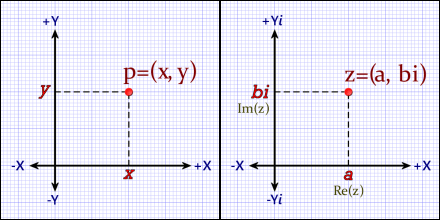
Cartesian plane (left) and the complex plane (right). Both are two-dimensional Euclidean coordinate spaces. A point, p, has an (x,y) coordinate. A complex number, z, is similar, but has a real part, a, and an imaginary part, b.

Note however that, in quantum mechanics (and in math in general), the concept of orthogonality generalizes beyond the intuition of right angle to the more important concept of linear independence (another term is degrees of freedom).

§

Given a coordinate space with points, we derive the notion of a distance between two points.

Consider a simple space, the one-dimensional real number line. In this space, each point is a real number, and its coordinate is that number. (The point is right on top of its “shadow”, so to speak.) The space has only one dimension, so the coordinate has only one component.

The distance between two points on the line is their difference — one number minus the other.

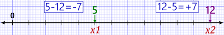
One-dimensional coordinate space — the real number line.

But hang on, there’s a wrinkle. Let’s say one point is 12 and the other is 5. The difference going one way is +7, but going the other way is -7. Is that really what we want when we speak of “distance” between points?

In some cases, yes, the sign tells us which way we’re going, but as a general concept we don’t refer to distance with negative values — there’s no such thing as a negative distance. (Except abstractly as a debit; “miles to go before I sleep.”)

What we can do is take the square root of the square.

Then we always get a positive number.

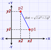
Figure 1. Euclidean Distance

This is the foundation of the Pythagorean notion of distance in a Euclidean space.

We square the distances projected by the points on each axis, add those squares together, and then take the square root of the sum. It’s the same thing we just did with the one-dimensional number line, but extended to multiple dimensions.

Note that the squaring means it doesn’t matter in which order we subtract one from the other. Any negative value we get gets squared away, so we only sum positive distances.

In two dimensions, of course, this reduces to the famous Pythagorean theorem from high school geometry, but it applies to any number of dimensions.

For instance, in three dimensions:

Where (x,y,z)₁ and (x,y,z)₂ are any two points in 3D space.

You may not have thought of the Pythagorean theorem as a measure of distance between points, but that’s what it really is, a generalization of distance in a coordinate space. That’s why its form shows up in other contexts; standard deviation, for instance.

§ §

A vector space is a coordinate space where we imagine an “arrow” (a vector) from the origin to each point in the space. (The origin is the single point in the space where the coordinate components are all zero.)

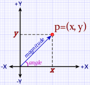
Figure 2. A Vector

While a coordinate space is an infinite density of points, a vector space is an infinite bristle of vectors all pointing out of the center, one vector per point.

(There are other types of vector spaces where the arrows don’t all start at the origin, but we’re not concerned with those here.)

Along with the idea of a distance between two points, a vector space allows some additional concepts:

Firstly, the arrow implies a distance from the origin to the point — a length to the arrow. We use the distance equation which, since the origin’s coordinates are all zero, simplifies to:

We call this distance the magnitude or Euclidean norm of the point.

Note that there is a zero vector (all zeros), which has magnitude=0. All other vectors have a magnitude greater than zero.

Secondly, the arrows in a vector space imply an angle between any two vectors or between any vector and any axis (an axis is an implicit vector).

Vectors and angles allow an alternate coordinate system, called polar coordinates, that identifies points by their angle and magnitude:

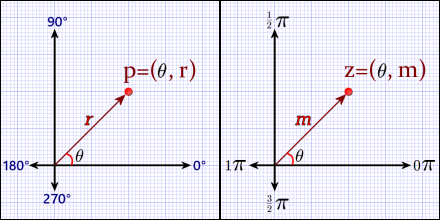
Polar coordinate systems for cartesian plane (left) and the complex plane (right). Axes shown in degrees (left) and radians (right) are interchangeable. A cartesian polar point, p, has an angle, θ (theta), and a radius, r. A complex point also has an angle, but her the vector length is the magnitude, m.

As a 2D vector space, the complex plane sees every complex number as a vector. Each has a magnitude and an angle (or argument) relative to the positive X-axis. Therefore the complex plane has a kind of built-in polar mapping.

Among other things this means:

For any complex number z with angle theta (θ) and magnitude eta (η).

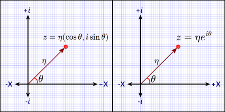
Complex plane using trigonometric coordinates (left) and exponential coordinates (right). The normalization constant, η (eta) is the Euclidean norm of z. The exponential version has the advantage of being easy to use as a rotation operator.

These identities are extremely important in quantum mechanics (and in wave mechanics in general). [Especially the exponential form (right-hand side above). See Circular Math and Fourier Geometry for details.]

To get η and θ from some complex number z:

[One tip about quantum math: learn the Greek alphabet. I use eta here because the η looks like an ‘n’ so it’s often used for the ‘normalizing’ constant. Theta is very commonly used for an angle. There is also that eta and theta are alphabetically adjacent, and similar sounding, so they make a cute couple.]

§

Figure 3. Inner Product

The notion of an angle between two vectors lets us define the idea of an inner product (also known as a dot product). This operation encodes both the angle and the magnitude of the vectors in the scalar result.

Algebraically, we take the two vectors multiply the respective components of their coordinates together and then sum those products.

For example, in Figure 3:

v = (1.0, 1.5), u = (3.0, 1.0)

So their inner product is:

v·u = (1.0 × 3.0) + (1.5 × 1.0) = 3.0 + 1.5 = 4.5

Note that the inner product of a vector with itself is the norm squared:

v·v = (1.0 × 1.0) + (1.5 × 1.5) = 1.0 + 2.25 = 3.25 = |v|²
u·u = (3.0 × 3.0) + (1.0 × 1.0) = 9.0 + 1.5 = 10.5 = |u|²

Because an inner product is: x²+y²+z²… That should look familiar as part of calculating the Euclidean distance.

§

Geometrically, an inner product is an orthogonal projection of one vector onto the other. The inner product is the length of the projection times the length of the other vector.

In Figure 3, p is the projection of vector v onto vector u. The length of that projection is the cosine of the length of v (because there is a right-triangle from the origin to p to v). The inner product is p times the length of u:

Where θ is the angle between the vectors. The inner product is important enough that I’ll return to it in the future.

§ §

The intent here is that two-dimensional spaces offer some intuition about spaces with higher dimension. In some cases, a space can have an infinite number of dimensions. A very large number isn’t uncommon.

The need for many dimensions is hinted at by a phrase I used above: “degrees of freedom.” Each degree is a dimension, and here’s where things start to get a bit involved.

In three-dimensional space — our physical space — every particle has a 3D location coordinate and a 3D momentum or energy vector. Therefore, every particle has six degrees of freedom and requires six dimensions to specify. A two-particle system requires 12 dimensions since the particles are independent.

In classical mechanics, there is no quantum uncertainty, and the position vector, r, and the momentum vector, p, precisely specify the system.

In quantum mechanics, uncertainty changes the equation (literally, from Newton’s to Schrödinger’s), but in three dimensions we still need six numbers for two vectors. In this case we deal with position and energy potential.

To reduce the complexity, and because the math is essentially the same, most quantum mechanics instruction begins with one particle and one dimension. Physical dimensions interact, so it’s not as simple as just doing the math three times, but the principles are the same.

§ §

Next time: linear transforms and operators (and matrices, oh my). That’s looking like two posts, one for transforms, one for operators.

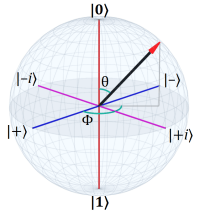
Down the road: quantum states, eigenvectors and eigenvalues, the Bloch sphere, and spin. As I mentioned in the Introduction, the ultimate goal is exploring the Bell’s Inequality experiments.

These posts will build on previous ones, so be sure to ask about anything you don’t fully understand — it may be important later.

Stay vectored, my friends! Go forth and spread beauty and light.

∇