 This reference page just iterates the basics of Matrix multiplication. See the Matrix Math post for additional information. See the Quantum Qubit Math page for examples of matrices in use in basic quantum mechanics.
The Basic Rule of Matrix Multiplication: The number of columns in the first matrix (the one on the left) must match the number of rows in the second matrix (the one on the right). This is always true when both matrices are square and have the same size. It’s when they aren’t that you have to be aware of this rule.
So: if A and B are both matrices, then when A×B, the number of columns in matrix A must match the number of rows in matrix B.
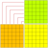
The diagram in the upper right symbolizes this. The orange squares represent matrix A (the left-hand one), and the green squares represent matrix B. The yellow squares represent the result matrix. The red lines indicate how the columns of the orange matrix must match the rows of the green matrix.
For example:
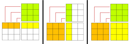
The above (from left to right) illustrates multiplying: [1×3] and [3×3] matrices (the result is a [1×3] matrix); [3×3] and [3×1] matrices (the result is a [3×1] matrix); and two [3×3] matrices (the result is another [3×3] matrix).
You can apply the Basic Rule and this visualization to the examples below.
[1×1] times [1×1]
We start with the special (degenerate) case of a [1×1] matrix times another [1×1] matrix. While mathematically legal, there isn’t much application for [1×1] matrices, but they do represent an edge case for matrix multiplication. The result is a [1×1] matrix. Its single value is the same as we’d get multiplying two scalars together:

But note that a [1×1] matrix is not a scalar. (The difference becomes obvious in the next two cases.)
[1×1] times [1×2]
Another special case, similar to the first case in using a [1×1] matrix but multiplying it here against a [1×2] matrix (a row vector). The result is another [1×2] matrix:

As in the first case, the result amounts to multiplying the row vector by a scalar (giving us a scaled version of that row vector):

But note that, unlike the scalar multiplication, the matrix multiplication cannot be reversed because [1×2][1×1] is an illegal operation. (The number of columns in the first matrix doesn’t match the number of rows in the second.)
Bottom line, a [1×1] matrix is not (always) the same as a scalar!
[2×1] times [1×1]
Yet another special edge case. Here’s the legal version of putting the “scalar” matrix second. In this case, the single column of the [2×1] matrix (a column vector) matches the single row of the [1×1] matrix:

Again, the result amounts to multiplying the column vector by a scalar (giving us a scaled version of that column vector):

However, as in the [1×1][1×2] case above, the [2×1][1×1] operation cannot be reversed (due to column/row mismatch), whereas with the scalar operation it can. So, once again, a [1×1] matrix is definitely not the same as a scalar.
[1×2] times [2×1] (inner product)
Multiplying a row vector by a column vector results in a [1×1] matrix usually treated as a scalar value called the inner product:

In Dirac’s Bra-Ket notation, generally speaking, a bra is row vector, and a ket is a column vector (see Bra-Ket Notation for details). Often the bra is the complex conjugate transpose of a ket. For example, given the quantum state:

Where α is a complex number, then:

Where α* is the complex conjugate of α.
[2×1] times [1×2] (outer product)
Multiplying a column vector by a row vector results in a matrix with as many rows and columns as the vectors (in this case, a [2×2] matrix):

This is known as taking the outer product.
In Bra-Ket notation, this is (using the definition of |Ψ〉 above):

Which, among other things, allows the definition of quantum gates in terms of combinations of state vectors. Such gates are always square matrices.
[2×2] times [2×2] (square matrix multiplication)
Multiplying two (same-sized) square matrices results in a new matrix of the same size (in this case, [2×2]):

(Multiplying square matrices is what many think of as “matrix multiplication” but as the many examples here show, it’s not the only form.)
[2×2] times [2×1] (column vector transformation)
One crucial operation is multiplying a square matrix (in this case [2×2]) times an appropriately sized column vector (specifically, a [2×1] matrix). The result is another column vector transformed by the values of the first matrix (an “operator”):

This is a common operation in quantum mechanics (and linear algebra in general). Vectors (or quantum states) are typically represented as column vectors. Square matrices act as operators on those vectors, transforming them into new (column) vectors. [See Linear Transforms for more details.]
[1×2] times [2×2] (row vector transformation)
The flip side of the above (and just about as crucial) is multiplying a row vector times a square matrix. Note that the row vector must come first. The result is another row vector transformed by the square matrix:

This is the matching operation to the column vector transformation above but for row vectors. In quantum mechanics, these two transformations are represented as:

Where Ô is an operator (a square matrix) and |Ψ〉 is a quantum state (column vector). [See What’s an Operator? for more details.]
[1×1] times [1×3]
Moving on to matrices with three rows and/or columns, for thoroughness we start with the two edge cases involving a [1×1] matrix. The first calls for a [1×3] row vector:

As in the above example with [1×1][1×2] multiplication, the result is the same as if we’d multiplied the [1×3] matrix by a scalar value:

This extends to multiplying a [1×1] matrix times any [1×N] row vector.
[3×1] times [1×1]
The other edge case, where the [1×1] matrix comes second, requires a [3×1] column vector:

Again, this is the same as multiplying the column vector by a scalar value:

This extends to multiplying any [N×1] column vector time a [1×1] matrix .
[1×3] times [3×1] (inner product)
As with the [1×2][2×1] example above, multiplying a row vector by a column vector results (technically) in a [1×1] matrix that is usually treated as a scalar value:
![\begin{bmatrix}{a}_{11}&{a}_{12}&{a}_{13}\end{bmatrix}\begin{bmatrix}{b}_{11}\\{b}_{21}\\{b}_{31}\end{bmatrix}=[{a}_{11}{b}_{11}+{a}_{12}{b}_{21}+{a}_{13}{b}_{31}]](https://s0.wp.com/latex.php?latex=%5Cbegin%7Bbmatrix%7D%7Ba%7D_%7B11%7D%26%7Ba%7D_%7B12%7D%26%7Ba%7D_%7B13%7D%5Cend%7Bbmatrix%7D%5Cbegin%7Bbmatrix%7D%7Bb%7D_%7B11%7D%5C%5C%7Bb%7D_%7B21%7D%5C%5C%7Bb%7D_%7B31%7D%5Cend%7Bbmatrix%7D%3D%5B%7Ba%7D_%7B11%7D%7Bb%7D_%7B11%7D%2B%7Ba%7D_%7B12%7D%7Bb%7D_%7B21%7D%2B%7Ba%7D_%7B13%7D%7Bb%7D_%7B31%7D%5D+&bg=f9fbf9&fg=00007f&s=0&c=20201002)
The Bra-Ket notation mentioned extends to vectors of any size. In this case, the quantum state would be defined:

But the vector could have as many rows as required. Likewise, the inner product operation applies to multiplying row vectors times column vectors of any size (so long as they have matching sizes).
[3×1] times [1×3] (outer product)
Multiplying a column vector times a row vector, as in the [2×1][1×2] example above, results in a square matrix, but in this case a [3×3] matrix:

The outer product operation also extends to column and row vectors of any size (presuming their sizes match).
[3×3] times [3×3] (square matrix multiplication)
Of course, we get a [3×3] matrix when we multiply two [3×3] matrices:

Which is a bit of a squeeze! (And why we’ll stop at [3×3] matrices, but the general ideas shown for these apply to matrices with larger dimensions.)
[3×3] times [3×1] (column vector transformation)
The [3×3][3×1] case of using a square matrix to transform a column vector is essentially the same as the [2×2][2×1] case above. The only difference is the addition of the third index (row in the vector, row and column in the square matrix):

As with other examples, this extends to any [N×N][N×1] case where a square matrix transforms a column vector.
[1×3] times [3×3] (row vector transformation)
The [1×3][3×3] case of transforming a row vector with a square matrix is also essentially the same as the matching [1×2][2×2] case above:

And, of course, this also extends to any [1×N][N×N] case where a row vector is transformed by a square matrix.
Identity Matrix
For a given operation (such as addition or multiplication), using the identity operand for that operation just returns the other operand. With scalar addition, the identity is zero because x+0=x. In scalar multiplication, the identity is one because x×1=x. If the operation is rotation, then in the general case, the identity is a rotation of 360° because that (usually) leaves whatever is being rotated looking the same.
Matrix addition (which requires matrices of the same size) just adds elements, so the identity matrix for addition is the zero matrix. The actual matrix required depends on the number of dimensions. For three, the zero matrix is:

Matrix multiplication (remember the Basic Rule about rows and columns) doesn’t have the one-to-one aspect matrix addition has, so the identity matrix for multiplication is a bit less obvious (it’s not just all ones). Again, the actual matrix depends on the number of dimensions (but it must be square). For three dimensions, the identity matrix is:

Whatever size is necessary, the identity matrix is square with all zeros except for ones in the main diagonal. Multiplied with another matrix, the result is that other matrix. Note that, so long as the Basic Rule is followed, the other matrix can have a variety of sizes. In particular, one can multiply them with row and column vectors:

The order depends on whether one has to match rows or columns with the identity matrix. In the case of another (obviously) same-sized matrix, the order doesn’t matter:

Note that matrix multiplication usually is not typically commutative, but when one operand is the identity matrix, then it is.
Matrix Transpose
The transpose of a matrix is copy of that matrix that has been flipped along a diagonal line starting in the upper-left and extending to the lower-right. If the matrix is square, the result is square. If the matrix is not square, the result has the number of rows and columns swapped.
Given the matrix M:

The transpose is:

In the case of a non-square matrix (column vector) V:

The transpose is:

In Bra-Ket terms, this transforms the ket |V〉 to the bra 〈V|. The reverse, transposing a row vector to a column vector, turns the bra 〈V| to the ket |V〉.
(Note that usually bras and kets use complex numbers, so the transpose required is the complex conjugate transpose — each number not on the transpose diagonal becomes its complex conjugate.)
Matrix Trace
The trace of a matrix — it must be a square matrix — is simply the sum of the elements along the main diagonal (the one from the upper-left to the lower-right).
Given the matrix M:

The trace is:

The trace of a matrix is the sum of its eigenvalues.
Matrix Determinant
The determinant of a matrix — it must be a square matrix — is a scalar value that characterizes certain properties of the matrix and is associated with matrix eigenvectors and eigenvalues.
Calculating it for a [2×2] matrix is simply:

Calculating it for a [3×3] is a bit more involved.

Which looks messy and weird until you study it. There are six groups of triple multiplications. Three are added; three are subtracted. Each group consists of three matrix values taken in diagonals. The three that run left-to-right (top-to-bottom) are the ones added, the three that run right-to-left are subtracted.
Calculating it for [4×4] and higher matrices is even more involved. See the Wikipedia article for details.
Matrix Inverse
The inverse of a matrix — it must be a square matrix — is another (square) matrix such that the matrix times its inverse gives the identity matrix:

In the appropriate dimension, of course. Here’s an example in two:

As with the determinant, calculating a matrix’s inverse can get involved with higher dimension matrices. See the Wikipedia article for details. For [2×2] matrices, there is a simple formula:

Which uses the determinant function above. Using the trace function from above, it can also be calculated:
![{M}^{-1}=\frac{1}{\textsf{det}({M})}\left[\textsf{trace}({M})\mathbb{I}-{M}\right]](https://s0.wp.com/latex.php?latex=%7BM%7D%5E%7B-1%7D%3D%5Cfrac%7B1%7D%7B%5Ctextsf%7Bdet%7D%28%7BM%7D%29%7D%5Cleft%5B%5Ctextsf%7Btrace%7D%28%7BM%7D%29%5Cmathbb%7BI%7D-%7BM%7D%5Cright%5D+&bg=f9fbf9&fg=00007f&s=0&c=20201002)
Making it pretty simple to calculate the inverse for [3×3] matrices. As mentioned above, the determinant function for higher dimensions gets messier, and so does calculating the inverse.
But doable when necessary.
Matrix Eigenvectors
Square matrices that act as operators on vectors can have eigenvectors and associated eigenvalues. If, for certain vectors, a transformation scales but doesn’t rotate them, those vectors are eigenvectors of that transformation. The amount they are scaled is their associated eigenvalue. Note that eigenvectors can be scaled by +1 — which leaves them completely unchanged — or by a negative number, which, in addition to scaling them, reverses their direction.
This is expressed in the equation:

Where M is a square matrix acting as an operator, V is a column vector, and lambda (λ) is a scalar value that scales V. Expressed in terms of, say, a [2×2] operator and a [2×1] column vector:

I may expand on this someday, but for now, see the Eigen Whats? post for more info (especially the comment section).
See also:
Spacetime Matrix: Using a matrix to implement how relativistic speeds distort spacetime under Special Relativity. [From the Special Relativity series.]
Ø


And what do you think?