February 27, 2026

Dual Numbers and Why 0!=1

Recently, I learned an interesting new math trick involving what are known as dual numbers. These are compound numbers similar in form to complex numbers but with a different kind of “magic” element enabling their behavior.

What makes them interesting to people like me is the surprising way they provide a fast and easy technique for software to generate the derivative of a given function.

As an unrelated bonus, a simple explanation of why zero-factorial is equal to one rather than zero (which might seem more intuitive).

Dual numbers look a bit like complex numbers:

$\textsf{complex:}\;{z}=({a}+{bi})\qquad\textsf{dual:}\;{d}=({a}+{b\epsilon})$

They share the same (a+bx) binomial form where a and b are real numbers and x is something special.

In complex numbers, x is the “magic” number i, which is defined:

${i}=\sqrt{-1},\quad{i}^{2}={-1}$

In dual numbers, x is the “magic” number epsilon, usually denoted ε, which is defined:

$\epsilon\ne{0},\quad\epsilon^{2}={0}$

Which makes them a little weird. No number squared is zero except zero, but epsilon is explicitly not zero.

Complex numbers have a real part and an imaginary part. Dual numbers have a real part and an epsilon part.

Addition and multiplication work as they do with any binomial.

Addition adds the two parts separately:

$({a}\!+\!{b\epsilon})+({c}\!+\!{d\epsilon})=({a}\!+\!{c})+({b}\!+{d})\epsilon$

Multiplication uses the usual FOIL method (first, outside, inside, last):

$({a}\!+\!{b\epsilon})\times({c}\!+\!{d\epsilon})={ac}+{bc}\epsilon+{ad}\epsilon+{bd}\epsilon^{2}$

Which, because epsilon squared is zero, reduces to:

$({a}\!+\!{b\epsilon})\times({c}\!+\!{d\epsilon})={ac}+({bc}+{ad})\epsilon$

Giving us another dual number. (Just like multiplying two complex numbers results in a new complex number.)

And that’s it. That’s dual numbers.

No doubt fascinating to mathematicians for the mathematical properties, but what makes them interesting to computer programmers is how they allow us to calculate the derivative — aka the instantaneous slope of the curve — of a function.

Let’s start with a simple example:

${f}({x})={x}^{2}$

We have a function, named f, that squares x — any value we give it. Such a simple function has a simple derivative:

$\frac{d}{dx}{f}({x})={2x}$

Now look what happens if we give f a dual number x+ε:

${f}({x}\!+\!\epsilon)=({x}\!+\!\epsilon)^{2}=({x}\!+\!\epsilon)({x}\!+\!\epsilon)={x}^{2}+{2x}\epsilon+\epsilon^{2}$

Which because of epsilon magic reduces to:

${f}({x}\!+\!\epsilon)={x}^{2}+{2x}\epsilon$

Notice something interesting. This result divides into two parts: the original function (x²) in the real number part on the left and the derivative (2x) in the epsilon part on the right.

Let’s try a more interesting example:

${f}({x})={2}{x}^{2}-{7}{x}+{5}$

The expected derivative is 4x-7.

If we give the function x+ε:

${f}({x\!+\!\epsilon})={2}({x\!+\!\epsilon})^{2}-{7}({x\!+\!\epsilon})+{5}$

This works out to:

${f}({x\!+\!\epsilon})={2}({x}^{2}+{2x}\epsilon)-{7x}-{7}\epsilon+{5}$

Which becomes:

${f}({x\!+\!\epsilon})={2}{x}^{2}+{4x}\epsilon-{7x}-{7}\epsilon+{5}$

We regroup this into:

${f}({x\!+\!\epsilon})=\left({2}{x}^{2}\!-\!{7x}\!+\!{5}\right)\,+\,\left({4x}\!-\!{7}\right)\epsilon$

And there it is again. The real number part on the left is the original function, and the epsilon part on the right is the derivative. Neat trick.

It works by equating epsilon with the tiny incremental dx of the derivative. Recall that values smaller than one become even smaller when squared. For instance, ½ squared is ¼.

In epsilon we have a quantity that is explicitly not zero, but which squares to zero. It’s as if epsilon is almost but not quite zero, and when squared it becomes so tiny that it effectively vanishes.

Note that the squares of very small quantities get exponentially smaller than the quantities. For example, the square of 1/100 is 1/10000. For every zero in the first number, add two zeros in the second. So, a vanishingly tiny value, when squared, could (at least symbolically) become a beyond-vanishing quantity, i.e. zero.

Epsilon is effectively the “magical” infinitesimal.

Programmers can leverage dual numbers in languages that allow user-defined data types. The idea is that one defines a dual-number data type that acts like a number. That is, it handles math operations such as add, subtract, multiply, divide, and exponentiation. The more math operations it handles, the more versatile will be the data type.

A typical use case might involve an app that takes inputs defining a mathematical function and outputs a graph of that function along with a graph of its derivative.

For example, suppose we graph the function above, 2x²-7x+5:

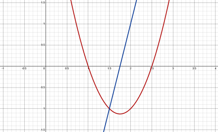
The red line graphs the function; the blue line graphs its derivative.

Graphing the function involves generating a bunch of x values and passing each to the function to get the y value at that point. Essentially, we iterate over the horizontal axis above. The smoothness of the curve depends on how finely we divide the x values. For example, if we use the numbers visible in the image along the X-axis, we’d get the following y values:

X value	Y value
-1.0	+14.0
-0.5	+9.0
+0.0	+5.0
+0.5	+2.0
+1.0	+0.0
+1.5	-1.0
+2.0	-1.0
+2.5	+0.0
+3.0	+2.0
+3.5	+5.0
+4.0	+9.0

But the graph wouldn’t look very smooth:

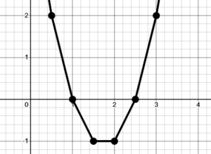
So, we obviously want to generate lots of closely separated points to get a smooth graph.

More to the point (pun unintended), we generate the derivative by creating dual numbers for each x value. We pass x+ε to the function rather than just x.

For each x+ε value we give the function, we get back a dual number result. We use the epsilon part of that returned value as the derivative value (the real part is the function value, so this lets us graph both curves in one pass).

Bottom line, when we give the function dual number x values, we get back a pair of values: the function’s value at that x point and also its derivative at the same point. Two for one.

It’s a handy trick for programmers. There are normally two ways to generate the derivative of a function. Firstly, calculate the actual derivative. This isn’t too hard to automate for basic polynomials, but it gets harder for more complex functions. It does have the advantage of being exact. When we use a calculated derivative function, we get back precise true values.

Secondly, we can generate the y values for the function and use adjacent ones to derive the slope of the curve at that point. This has the advantage that the complexity of the function doesn’t matter. On the other hand, it’s an approximation. The derived curve won’t be precise and true.

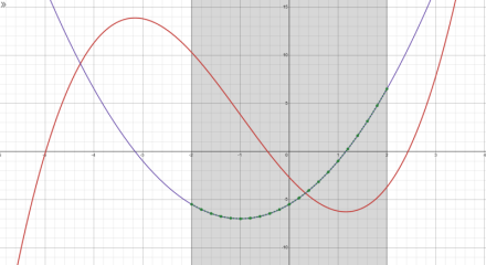
The red curve is a function; the blue curve is its derivative. Both are mathematically calculated. The green dots are points calculated using dual numbers with the function. An exact match!

Dual numbers provide a third option that’s easy to do (once you create your dual number data type) and precise and true. The derivative values we get this way are the actual values as if from a calculated derivative.

So, yeah, handy trick for the toolkit.

[For a Python implementation of dual numbers, see this post.].

§ §

As a bonus today, have you ever wondered why zero-factorial is one rather than the perhaps more intuitive zero?

The lede image makes it seem even more like it should be zero. Then the numbers would match on both sides. But if we zoom out a bit:

${5}!={120}\\[0.2em]{4}!={24}\\[0.2em]{3}!={6}\\[0.2em]{2}!={2}\\[0.2em]{1}!={1}\\[0.2em]{0}!={1}$

We see a different pattern. If we use the usual definition of factorial to try to determine what zero-factorial should be, we immediately see a problem:

${n}!=({n})({n\!-\!\!1})({n\!-\!\!2})\ldots({1})$

We can’t include zero in that definition because it would make all factorials equal to zero.

If we ‘spell out’ the factorials above, we see a second problem:

${5}!={5}\cdot{4}\cdot{3}\cdot{2}\cdot{1}\\[0.2em]{4}!={4}\cdot{3}\cdot{2}\cdot{1}\\[0.2em]{3}!={3}\cdot{2}\cdot{1}\\[0.2em]{2}!={2}\cdot{1}\\[0.2em]{1}!={1}\\[0.2em]{0}!={?}$

What do we put for zero?

Because of this, some mathematicians consider zero-factorial to be undefined.

But we find a definition if we look at the factorial values and consider what it takes to get from one factorial to the previous one:

${5}!={120}\div{5}={24}\\[0.2em]{4}!={24}\div{4}={6}\\[0.2em]{3}!={6}\div{3}={2}\\[0.2em]{2}!={2}\div{2}={1}\\[0.2em]{1}!={1}\div{1}={1}\\[0.2em]{0}!={1}$

We can’t continue because we would have to divide one by zero, so this pattern ends with zero-factorial. We cannot do factorials with negative numbers.

But we can show that 0!=1.

§ §

Dual numbers; dual topics. 😄

Stay dual, my friends! Go forth and spread beauty and light.

∇

About Wyrd Smythe

The canonical fool on the hill watching the sunset and the rotation of the planet and thinking what he imagines are large thoughts. View all posts by Wyrd Smythe

This entry was posted on Friday, February 27th, 2026 at 9:14 am and tagged with computer programming, derivatives, dual numbers and posted in Computers, Math. You can follow any responses to this entry through the RSS 2.0 feed.