Sideband #79: Growth Curves

nx vs xⁿ vs n^x (for n=42)

You’ve probably heard the phrase “exponential growth” in reference to something that grows very fast. A common example is bacteria in a petri dish. More relevant in daily life, perhaps, the spread of a highly communicable disease or a “viral” meme. These things all can have exponential growth.

You may also have heard the phrase “geometric growth” and wondered how — if at all — it differs from the exponential form. Recently I found myself curious enough about the difference to dig into it a little and find out once and for all.

This post records my simple exploration.

The punchline is that exponential growth and geometric growth are almost the same thing (some even treat them as identical). The former is the general case with broad application while the latter is the more specific case for discrete units. The examples listed in the first paragraph all involve such units (bacteria, infected people, memes shared) and are examples of geometric (exponential) growth.

Geometric growth is also known as geometric progression, sequence, or series. Regardless of the exact terminology, a geometric progression is a list of non-zero numbers where each next number in the list comes from multiplying the previous number by a fixed (non-zero) number, called the common ratio. The general form is:

Where r is the common ratio and a is the scale factor (and is equal to the sequence’s starting value and must be non-zero). In general, for the nth term in the sequence:

As an example, suppose the progression starts at five (a=5) with common ratio of three (r=3). Then we have:

Evaluating the various powers of r gives us:

Multiplying the terms, the geometric progression (or sequence or series) is:

The discrete values of a geometric series make it a natural for a bar chart:

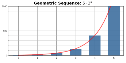
Figure 1a. A geometric sequence with a=5 and r=3.

The values get very large quickly — the basic characteristic of exponential growth. Figure 1a, with only six steps of the sequence, barely registers the first value (of 5) while the last value (1,215) goes above the chart.

Figure 1a also shows (in red) the exponential curve behind the geometric progression (created by using 100 steps between each bar to simulate a continuous growth rate).

The exponential growth — and the resulting difficulty of showing it on a graph — suggests we are better off using a logarithmic scale for the vertical axis:

Figure 1b: A vertical log scale allows values up to 885,735!

Which allows us to show twelve steps of the progression (the last one has a value of almost one million). Note that with a logarithmic scale the growth curve and heights of the bars now follow a straight line. Exponential growth is linear when viewed logarithmically.

[Because a log scale grows exponentially, too. Which is why log scales can never start at zero. The initial value of any exponential growth must always be non-zero.]

§

Exponential growth is the general case where some quantity changes over time at an ever-increasing rate. Mathematically, the derivative of an exponential function is always proportional to the function itself — which is not typical of derivatives of functions. Typically, the derivative of a function is a completely different function.

As a simple example:

The d/dx term is an operator that returns the derivative of the term following it, in this case the function x². (A function that returns the square of whatever value it’s given.) As the above shows, the derivative of the function x² is the completely different function 2x. (A function that returns double of whatever value it’s given.)

Jumping ahead a little, the quintessential exponential function involves Euler’s most famous constant, e=2.718281828… (forever; e is an irrational, in fact transcendental, number). Part of the magic of e is that it is its own derivative:

Which is not true of any other function, including other exponential functions, which all have proportional derivatives. In the case of e, though, the constant of proportionality is one. [For details on why, see the last section of this page.]

The general formula for exponential growth is:

Which you might recognize as the formula for compound interest.

The a with the subscript 0 (zero) is the initial value (similar to its appearance in geometric growth). In other words, the value at x=0.

The a with the subscript x is the function’s value at some later point (or time). Depending on requirements, x can be any continuous quantity in whatever units makes sense. Typically, x represents time (and is often denoted as t rather than x) but can be whatever applies to the situation (pressure or voltage, for instance). Note that x is not restricted to integer values; for example, x=1.333 is perfectly legit.

The r is, also as above, the growth rate, but notice how that growth rate is not only multiplied by the initial value (as above), but first added (“compounded”) to the current amount. It might make more sense seeing it with that starting value multiplied into the two values in the parentheses:

In the canonical case, where the starting value is one, the formula reduces to:

Which, when taken to a limit like this:

Gives us the value of Euler’s constant e (2.718281828…). Among its many features is that it’s the highest rate of return you can get with continuously compounded 100% interest. [See this page for details.]

[By the way: despite it seeming an obvious connection, e does not, in fact, stand for Euler. The story is that Euler tended to use vowels for his variables and happened to use e in this case. Over time it stuck. Another by the way: Euler is pronounced “Oiler”.]

§ §

That was a bit of a digression. The point is that exponential growth (and its discrete cousin, geometric growth) involves, as the name says, a formula with exponents.

But not just any formula with exponents, and this brings me to the second question I had regarding exponential growth. Specifically: what’s the difference between:

For some constant value n. Is there much difference? (Turns out: yes! They are, indeed, different types of growth rates.)

Going into all this, I wondered if the difference might be that the first one was geometric while the second one was exponential. As covered already: nope, geometric is a form of exponential. Which is the second one.

The first one is called polynomial growth. Crucially here, x is never an exponent. Rather, it’s the base number for a series of one or more numeric exponents, the highest of which denotes the order of the polynomial. We’ve already mentioned one of the simplest possible polynomial functions:

So simple it has a name: x-squared. (The function notation, the f(x)= part, serves as a reminder that x-squared is a function that takes a value.) Because the highest exponent is two, this polynomial has order two. Yes, “highest” because the terms of lower order are implied but have coefficients of zero. Written out fully, x-squared is really:

With coefficients: a=1 and b=0 and c=0. Even a high-order polynomial such as:

Implies all the lower-order terms (20 on down to 0) but with coefficients of zero.

Here are two even simpler polynomials (so simple we don’t really think of them as polynomials):

That first one, of course, includes the lower-order term x⁰ with a zero coefficient.

Here’s an example that might be more like your notion of a proper polynomial (of order three):

Nevertheless, all the examples above are “proper” polynomials! (Remember that the x term is really x¹ and the final term has an invisible x⁰, but these are rarely written out.) Here’s what that last polynomial looks like when graphed:

Figure 2: a polynomial (growth) curve with order three.

Figure 2 is immediately recognizable as an order-three polynomial due to its s-like shape. The coefficients will alter this shape significantly, even straightening out the wiggle, but the key aspect of an order-three polynomial is that it approaches (but never reaches) opposite signs of infinity as the positive and negative x values grow towards (but never reaching) their respective infinite values.

In contrast, our simple x² polynomial, which graphs as a parabola, approaches the same sign of infinity at both ends of the x-axis:

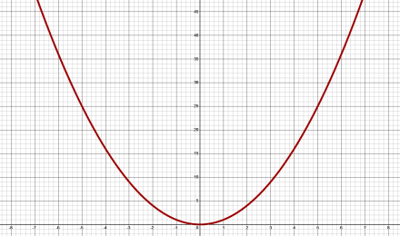
Figure 3. a polynomial grown curve with order two.

All even-order polynomials approach the same sign of infinity, whereas all odd-order polynomials approach opposite signs. Regardless, and this is the key point, all polynomials grow as x values increase. And almost always, we’re interested in how the curve grows along the positive x-axis. Typically, x=0 represents the beginning of the growth curve.

Lastly, the lower-order polynomials have generic names: order-two functions are called quadratic (or parabolic); order-three functions are called cubic; order-four functions are called quartic; and order-five functions are called quintic.

§ §

So, how does polynomial growth compare with exponential growth? The short answer is that exponential always wins. Eventually.

Depending on the numbers involved, it’s entirely possible for polynomial growth to reach larger values with low values of x. For example, here are the beginnings of the two curves for n=12:

Figure 4a. Curves for xⁿ (red) and n^x (blue) with n=12. Note the crossing at x=1.3122 where both curves have the value 26.07.

Figure 4a shows the initial stages of growth for an order-12 simple polynomial (red) and a basic exponential (blue). Based on the apparent trend so far, the red polynomial curve seems to be growing much more rapidly than the blue exponential one.

To show much more of these curves, though, we’ll first need to switch the y-axis to the logarithmic scale:

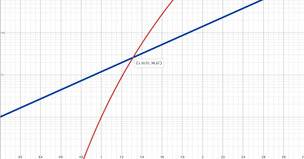
Figure 4b: Same as 4a but with a logarithmic vertical scale.

Which makes the blue exponential curve straight as it did with the plots in Figure 1b. Note that the crossing point is the same in both and that the relative slopes of the lines — the red one being noticeably steeper than the blue one — remains unchanged.

Something else becomes apparent in Figure 4b. The blue curve is straight, but the red curve now appears to bend towards the blue line. Which suggests it will cross it again at some point, but this time headed downwards.

Which is exactly what happens:

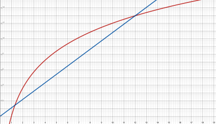
Figure 5. Curves for xⁿ (red) and n^x (blue) with n=12. Note the second crossing at x=12. Note also that the vertical scale goes to 10¹⁵!

As x grows, exponential growth always wins.

One thing we can notice about the respective curves is that:

As x increases along the x-axis, at some point it must equal n. At that value of x, the curves for polynomial and exponential growth cross. We can consider the slope of each curve at that point to determine how they cross. The one with the steeper slope is growing faster.

Of course, we’ve seen how the earlier crossing indicated the polynomial curve was steeper, so any conclusions we draw about x=n depend on the curves not crossing again. But n=12 gives us an even-order curve — a flat-bottomed parabola. So, there’s little reason to suspect the curve changes direction.

§

We can take the slopes of both lines by calculating their derivatives to give us numbers we can compare. Taking the derivative of the polynomial is simple:

Using the basic rule of derivatives:

Taking the derivative of the exponential is slightly more involved. An easy way is to leverage the ease of deriving exponentials using e and that an exponential in one base can be easily converted to an exponential in another base using the formula:

To convert 12^x to an exponential using e we can use the natural log (ln):

And deriving this is dead simple. For any value of n:

In this case, n=12, and ln(12) = 2.4849…, so:

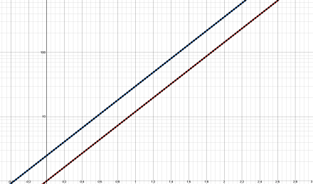
Figure 6. The exponential curve (red) and its derivative (blue). The derivative is the same curve but multiplied by a constant, ln(n). The black dots indicate alternate ways of calculating these curves as a self-check of the math discussed in the post.

Now we have our derivatives and can evaluate them at x=12:

And:

And (almost) nine trillion is certainly less than twenty-two trillion, so the exponential slope is greater than the polynomial slope at the crossing.

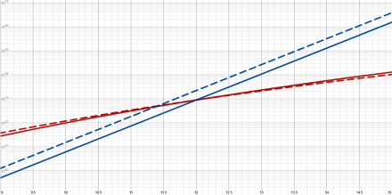
Figure 7. Closeup of the crossing at x=12, y=8,916,100,448,256. The dotted lines are the derivatives, and the blue derivative (exponential) clearly has a higher value than the red one (polynomial) at x=12 (see text for its exact value). Note that the polynomial derivative matches and crosses the polynomial curve at this point. The polynomial, its derivative, and the exponential all have the same value at x=12.

§

That we can convert any expression with an exponent to an exponential using e gives us a more direct way to compare the two functions. We can convert both to exponential expressions using e and compare them directly.

We converted the exponential above. Here it is again:

And here’s the polynomial expression converted to an exponential using e:

And, since e is the base in both, we just need to compare the exponent terms:

The left expression is some constant n times the (natural) log of x, and the right expression is x times the (natural) log of the constant n. Which is bigger?

We can graph the two expressions:

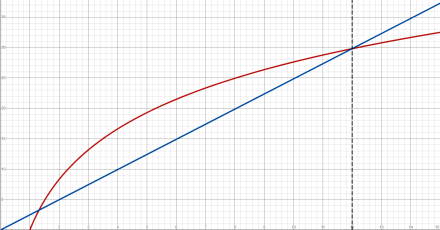
Figure 8: Just the exponential terms. Note the linear vertical axis!

And see the same behavior we saw in Figure 5. Note that the blue line (the exponential’s exponent) is linear (and so is the vertical axis). The term is just x times a fixed value, the log of n. But the red line is a constant value times the log of x, so the red line tends to flatten out.

Which means the blue line will always eventually go above it. So:

At least eventually. Ultimately, an exponential growth rate leads to larger numbers than a polynomial one (and both grow much faster than a linear growth rate).

§ §

We’ve talked about growth rates, but there can also be exponential decay, where an initially high value declines over time. A canonical example is the half-life of radioactive elements. Depending on the rate, growth can also be linear or essentially flat:

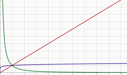
Figure 9. Linear (red), nearly flat (purple), and decaying (green).

The red line is a growth rate of 1.0, which results in linear growth. The purple line has a growth rate of 0.1, which results in almost no growth. Values closer to zero result in flatter and flatter rates. At zero, the curve is completely flat and there is no growth. The green line has a growth rate of -1.5 — negative values leading to exponential decay.

§ §

There’s a great deal more to talk about, but this has gone on long enough. Just for fun, one last graph:

Figure 10. Four curves: Linear, nx (black); Polynomial, xⁿ (red); Exponential, n^x (blue); and Super-Exponential, x^x (purple). The last three cross at x=30, y=30³⁰≈2.06×10⁴⁴.

The red polynomial and blue exponential curves are what they’ve been, but in Figure 10, n=30, so the crossing is at x=30. The black linear growth curve doesn’t hold a candle to even polynomial growth.

The “super-exponential” curve, x^x, which also crosses at x=30, has an even greater rate of grow than the others. Which makes sense considering the exponent terms of the normalized versions (that use e for a base):

The last term (for the super-exponential) grows with x times the log of x, which guarantees it eventually surpasses the other two (which x=n). (Note that it does not depend at all on the value of n.)

§ §

A classic puzzle illustrates a key aspect of exponential (in this case geometric) growth: The local pond supports the growth of water lilies. Left alone, the number doubles overnight. The town doesn’t want the pond entirely covered by water lilies — which will happen in 30 days. Because of busy schedules, the townspeople decide to wait until the pond is half covered before starting to clear the water lilies.

Given the 30 days until the pond is entirely covered, on what day do the townspeople need to get to work clearing it?

The information necessary to answer is supplied in the problem description.

Stay exponential, my friends! Go forth and spread beauty and light.

∇