X to the Zero Power

At some point in our early math education, we’re told that anything to the power of zero evaluates to one. 1°=1 and 5°=1 and 99°=1. Basically, x°=1 for all x. It’s typically presented as just a rule about taking anything to the power of zero, but it’s actually derived from a more basic rule about exponents.

Thinking about x° in connection with something else recently, it occurred to me there’s a second way to justify the notion that anything to the power of zero is one.

It also occurred to me 0ⁿ might be an implementation of the Dirac delta.

One can get through most math simply abiding by the rule that x°=1, but it can be derived from (what I consider) the single axiom about exponents:

It’s the one we learned first in school. When we raise something to some power, n, we calculate the product of that thing multiplied by itself n times. Using this axiom, we can derive an important theorem:

Anything to the power of one is just that thing. This is still a multiply operation, and the sense of multiplying by itself still applies. We’ll come back to that below.

We can also derive what is often presented as another (or sometimes the single) axiom:

Multiplying identical bases (the xs) is the same as adding the exponents on a single instance of that base. Because:

The two subgroups on the right are the same as the primary axiom above, so the two expressions are identical. Besides being useful in deriving further theorems, this equality lies at the heart of logarithms.

§

Now we can derive the equality x°=1. Start with:

We can use the theorem we just derived above to write:

We know that x¹=x, so we can rewrite the last two terms as:

Then we can divide both sides by x:

The xs cancel out leaving us with:

QED and Bob’s your uncle. (I, in fact, had an uncle named Bob.)

§ §

At least that’s one way to do it. This post exists because I thought of another. To understand it, we need to look under the hood of multiplication.

Addition is the core concept. If you have this, and you have that, you can add them together (and have either thisthat or tthhiast, depending on your preference). Basic and obvious. Multiplication is serial addition. You add this that many times (or that this many times).

[Exponentiation is serial multiplication (so serial-serial addition), but let’s stick with multiplication for the moment.]

More formally, both addition and multiplication are group operations that take two elements of the group (such as numbers) and produce a third (another number). There are some important requirements for group operations. A key one is that the operation has an identity element. When the identity element is used in the corresponding operation with another element, the result is always that other element.

For example, zero is the identity element for addition. Any number added to zero is just that number (0+x=x). Important in this case, one is the identity element for multiplication (1×x=x). Any number multiplied by one is just that number. (Obviously, 0+0=0 and 1×1=1.)

Note that identity elements depend on the group in question. For example, if the group is rotations in 3D, then the identity element is no rotation. (Group theory has a wide variety of applications.)

§

In a very real way, these group operations always begin with their identity elements. Think of zero as the initial buffer in which to add things during addition. One works as a similar buffer for multiplication. Zero wouldn’t work in this case because anything multiplied by zero is zero.

So, if we wanted to add 21 and 42, it theoretically breaks down like this:

Think of it as starting at zero, then sliding along the number line to 21, and then from there sliding 42 more units along the line to 63. Think of addition as two moves sliding through number space. Start by sliding from zero to the first number. Then, from there, slide as if from zero to the second number, make that same move but from where you are in number space.

Likewise, think of multiplication as two moves in number space but this time as scaling moves starting from one. For example, multiplying 21 and 42 starts at one and first scales (the number line) by 21 — it expands it by 21. Which scales 1 to 21. Now we scale it again, this time by 42 — everything expands by a factor of 42. This scales 21 all the way to 882 (21×42).

Multiplying by one leaves everything the same (which is why it’s the identity element). Multiplying by a number smaller than one reduces things, scales downwards. For instance, multiplying by 0.5 (½) reduces the scale by half— the 1 now scales to 0.5.

§

Deep theory aside, consider a basic algorithm for multiplication:

FUNCTION multiply (a, b):
    buffer = 0
    REPEAT b TIMES:
        ADD a INTO buffer
    RETURN buffer

This adds the input parameters a and b. The algorithm implements multiplication as serial addition, so the initial element in buffer is zero, the additive identity. The repeat loop adds the first parameter (a) to the buffer as many times as specified by the second parameter (b). Then it returns the result. Note that, if a=0 or b=0, then the result is zero.

Now consider a very similar algorithm for exponentiation:

FUNCTION power (a, b):
    buffer = 1
    REPEAT b TIMES:
        MULTIPLY a INTO buffer
    RETURN buffer

This raises base parameter a to the power of exponent parameter b. The algorithm implements exponentiation as serial multiplication, so the initial element in buffer is one, the multiplicative identity. Here the repeat loop multiplies parameter a as many times as specified by parameter b.

However, if the exponent parameter b is zero, then the loop is repeated zero times — which is to say not at all. So no multiplication takes place and the value returned is the initial value: one. a°=1.

[And if b is one, then then the loop is done just once, the initial buffer value of one is multiplied by a only one time. a¹=a]

Bottom line, the natural mechanism of exponentiation directly explains why x° is always one. The underlying mechanism of multiplication always initializes to one, and if the exponent is zero, we multiply the base times itself zero times (whatever that’s supposed to mean). All we have then is the initial buffer value.

§

The fly in the ointment is 0° — should it be, as shown above, equal to one? But how does something made of zeros evaluate to one? Generally, zero to the power of anything (0ⁿ=0 for all n) is still zero.

On the other hand, if we use the power algorithm above and set a=0 and b=0, the result returned is indeed one (weird as that seems). Plus, the rule and the logic behind it is pretty clear: x°=1.

So, which is right? Mathematically, neither. It’s generally viewed as undefined (same as with division by zero). There is no valid answer to 0°. But some number systems do treat it as valid and, depending on the system, give it the value of zero or one.

The Windows calculator is one system that treats it as valid and equates it to one (but, of course, all other powers of zero equate to zero as expected).

Under such a system, 0^x acts exactly like the Dirac delta function, δ(x). Both return zero for all x except x=0, in which case they return one. The function is zero everywhere with a single-value spike to one at zero.

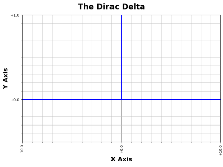
The spike can easily be shifted: the 0^a-x and δ(a-x) forms both shift the spike to a (because a–x=0 when x=a).

I found that interesting because the Dirac delta is sometimes taken as a kind of pretend function that works the way it does because mathematicians say so. It’s a kind of handy mathematical magic. But if you were to define it:

Then the function would be grounded in a mathematical reality.

Albeit perhaps a questionable one given the ambiguous status of 0°.

There is also that the Dirac delta does have a mathematical definition as an infinitely narrow Gaussian function, a bell curve squeezed horizontally until it’s just a spike. (In fact, if you read the Wiki page, you’ll see it has multiple mathematical definitions.)

And I suspect, validity of 0° aside, a bigger issue is that the mathematical definitions shown on the Wiki page can be integrated or differentiated, and I don’t think is true of 0ⁿ. But if all one wants is a simple function that vanishes everywhere — except for spiking to one at a given value (nominally zero) — then 0ⁿ does provide that.

§ §

Stay exponential, my friends! Go forth and spread beauty and light.

∇